DeepSeek OCR

Frontier AI Excel Blueprint

DeepSeek OCR was released last week. What’s the big deal?

Don’t we already have a lot of OCR tools that work well enough?

If you’re thinking this way, I hope this Blueprint and my explanation below can help you see its true significance, and prepare you for what’s next.

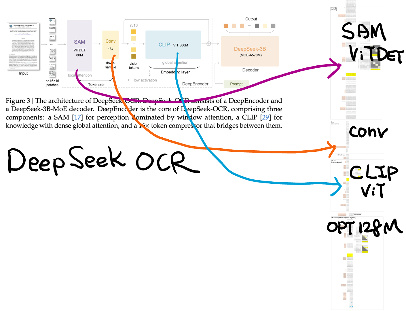
DeepSeekOCR stacks three Transformers into one tower.

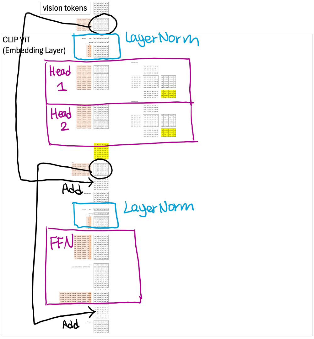
They all share a common backbone—pre-LayerNorm, multi-head attention, residual add, LayerNorm, and FFN with GeLU.

Below I use CLIP ViT to illustrate this common backbone.

But they differ in other ways, such as context size, attention mask and position embedding methods.

Why?

By the end of this long article, I hope you’ll have an intuition for these design choices—so you can make similar ones yourself in the future.

Another reason I like this topic is that it lets me compare real models. Whenever I say “this is from DeepSeek,” it grabs my students’ attention much more than “this came from an academic paper.”

👇 Scroll to the bottom to download the Excel Blueprint.

DeepSeek OCR Encoder

In this issue, I will focus on the Encoder, because that’s where most of the interesting design happens.

The decoder uses DeepSeek’s powerful new and large MoE model, mainly to train the Encoder. Last week I did a breakdown of its new DeepSeek Attention Layer.

My prediction?

People will soon start pulling out the DeepSeek OCR Encoder and plugging it into other downstream tasks.

The goal isn’t to build yet another OCR tool.

It’s to build a new visual encoder—one that’s not only as good as previous visual encoders but also reads, understanding what characters mean (local) and how they’re arranged (global). Moreover, it is doing all this very fast!

Training the DeepSeek OCR Encoder

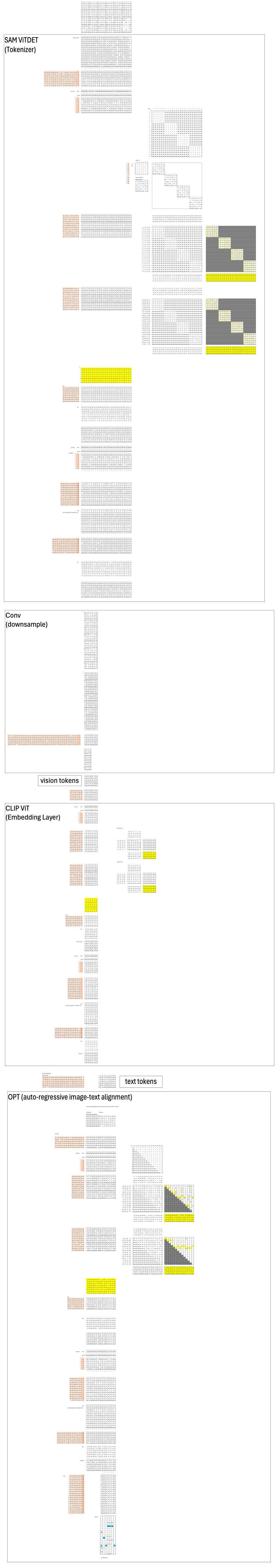
The DeepSeek OCR Encoder has three components:

1. SAM ViT — extracts local visual features

2. Convolution Layer — connects SAM-ViTDeT and CLIP-ViT

3. CLIP ViT — computes global visual features

A small transformer-based language model (Meta’s OPT) was used to align the joint embedding between visual and text modalities. Once training finishes, OPT is discarded.

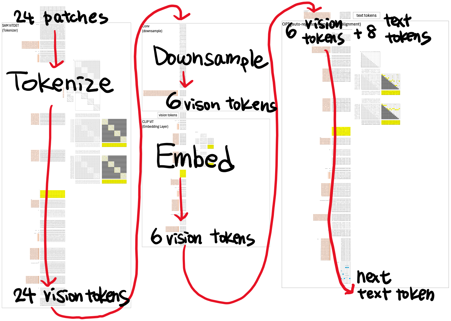
SAM ViT: Extract Local Visual Features

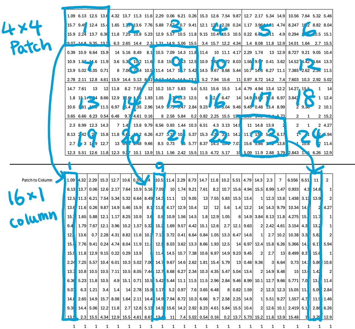
Input: a 16×24 image → divided into 4×4 patches → 24 patches total. Each patch becomes a column of 16 numbers—a token embedding that a transformer can process just like text.

SAM-ViTDeT comes from Meta’s legendary Segment Anything Model (SAM)—the model that practically ended half the PhD theses in segmentation. SAM-ViTDeT was trained to extract descriptive local features for downstream segmentation, so those features are perfect for reuse.

In my blueprint, the ViTDeT outputs 24 visual tokens, each an 8-D feature vector.

Convolution Layer

We need a connect SAM ViTDeT and CLIP ViT.

There are two challenges:

1. Their model sizes don’t match: 768 vs 512.

2. ViTDeT has too many tokens: 1024 by 1024. CLIP ViT can only handle 256 by 256 tokens.

In our blueprint, the version of these challenges are:

1. Model size: 8 vs 6

2. Tokens: 1024^2 vs 256^2

The convolution layer can deal with both challenges.

Reducing Tokens

Remember that SAM-ViTDeT outputs one token per image patch.

Each token contains 8 visual features describing that local region.

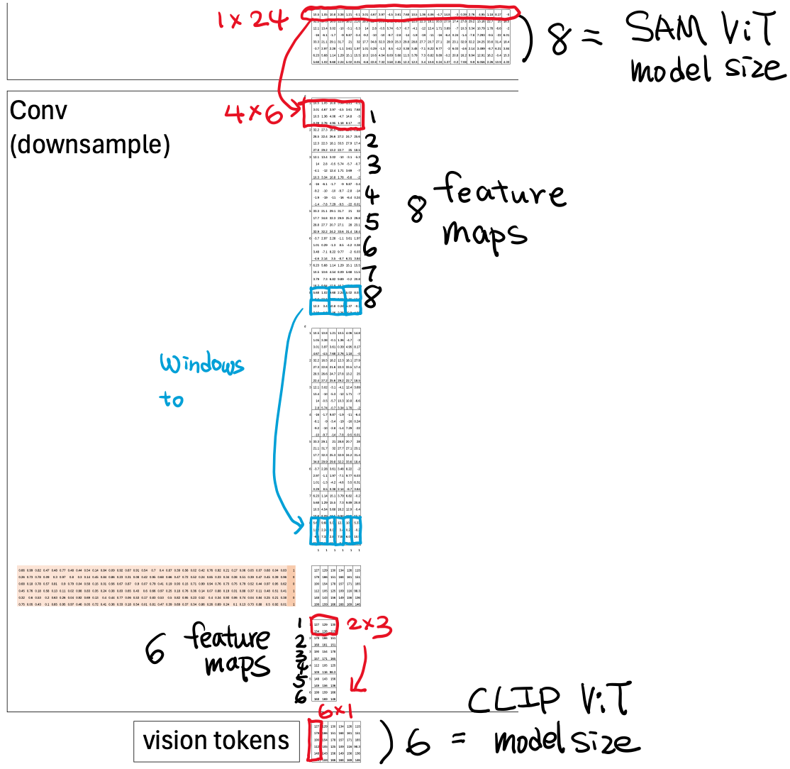
To visualize this, let’s take the first visual feature across all 24 tokens (a 1×24 vector, shown in red) and reshape it into a 2D feature map of 4×6—representing the spatial layout of those 24 patches.

Now we’ll run six non-overlapping 2×3 windows (shown in blue) across that map.
This operation is called “sliding windows,” although technically, nothing is sliding here. The term just helps you imagine how the windows cover the map.

Coincidentally, each window’s size (2×3 = 6) happens to equal the number of windows (6). I didn’t plan that—it just turned out that way when I built it all out by hand. So let me stress this: the window size and the number of windows don’t have to be the same.

In practice, we don’t slide these windows one by one using the CPU—that would be too slow. Instead, we reshape each window into a column vector, and likewise reshape and stack all the 2×3 kernels into rows (highlighted in red).

Once both windows and kernels are represented as columns and rows, we can hand them off to the GPU to compute the cross-correlation for all windows at once—through a single matrix multiplication.

No loops. No iteration. Just pure parallelism.

Reducing Model Sizes

So how do we go from 8 features down to 6?

Let’s zoom in on the convolution itself. Each window’s values are multiplied (or convolved) with a learnable kernel of the same 2×3 size (shown in red).

This kernel slides across every window—but crucially, we use the same kernel for all six windows within a feature map, keeping the operation consistent.

Since we have 8 input feature maps, we’ll need 8 kernels to generate one output feature.

Each kernel contains 6 weights (for the 2×3 window), so:

8 kernels × 6 weights = 48 parameters per output feature.

If we want to produce 6 output features, we repeat this six times—one row of weights per output channel—plus a bias term for each.

In matrix form, this looks like 6 rows × (48+1) columns, representing all learned parameters that convert 8-dimensional inputs into 6-dimensional outputs.

That’s the essence of the convolution layer—a compact, learnable bridge that not only reduces the number of tokens but also compresses feature dimensions so that CLIP-ViT can take over efficiently.

CLIP ViT: Compute Global Visual Features

The six vision tokens are then fed into CLIP-ViT.

When CLIP-ViT was first trained, its goal was to learn visual representations that align closely with text representations—so that images and their captions live in the same embedding space.

To achieve this, the model was trained on massive collections of image–text pairs, a process known as learning a joint embedding.

For DeepSeek OCR, the team built their own dataset of such pairs, and also drew extensively from LION, one of the largest open-source image–text datasets available, to strengthen this cross-modal alignment.

Inside CLIP-ViT, these six vision tokens attend to each other globally—every token can see every other token. Unlike SAM-ViTDeT, which restricts attention to local blocks, CLIP-ViT uses full self-attention to capture relationships across the entire image. This allows the model to combine local details into a coherent, global understanding of what the image represents.

In practice, each token becomes a mixture of information from all others, weighted by attention scores that reflect their contextual relevance. The result is a set of global feature vectors—compact yet expressive summaries that encode not only what each region looks like but also how all regions relate to one another. These global features are what make CLIP-ViT so effective for connecting visual data with language.

OPT: Learn Joint Embedding by Decoding

Once we have a set of visual tokens that capture both local features from SAM ViT and global features from CLIP ViT, the next step is to align them with the other modality—text.

In the original CLIP framework, this alignment was achieved through contrastive learning, that’s the “C” in CLIP. But DeepSeek OCR takes a different path: it replaces contrastive learning with an autoregressive decoding method, first proposed by Vary in 2023. This technique doesn’t just measure similarity; it generates text conditioned on the visual embeddings, creating a more fine-grained alignment between vision and language.

Before diving into how that works, it helps to recall how the original CLIP training operates.

Background: Contrastive Language-Image Pre-training

In CLIP, we take the six output vectors from the CLIP ViT and combine them—usually by averaging—to form a single image embedding vector, a compact summary of the entire image.

We do the same for the text: merge all the token embeddings (for example, words in a caption) into one sentence embedding vector by taking the mean.

Now we have both image and text represented in the same vector space, each as a single vector of equal dimension.

How do we compare them?

By computing their dot product—a simple measure of similarity between two vectors.

And when we’re working with thousands of image–text pairs at once, we perform many such dot products between all image and text embeddings.

How do we compute a lot of dot products efficiently?

Exactly—by turning them into a single matrix multiplication operation.

Predicting the Next Token: Alignment Through Generation

The autoregressive decoding method takes a very different approach from contrastive learning. Instead of comparing image and text embeddings to see if they match, it trains a small language model to generate text tokens directly from the visual embeddings—one token at a time.

At each step, the model predicts the next word based on all the previous words and the image features it has already seen. This sequential process mirrors how language models generate text, but now it’s guided by visual context.

You see, there are eight text tokens appended after the visual tokens. The model is trained to predict what the ninth text token should be, then the tenth, then the eleventh, and so on—comparing its predictions against the ground truth text from the training data. This process continues until it learns to generate text that accurately describes what’s in the image.

This setup forces the model to learn a deeper, step-by-step alignment between visual and textual modalities. It’s no longer just matching whole images to whole sentences—it’s learning how specific visual regions correspond to specific words or phrases.

In DeepSeek OCR, the OPT decoder plays this role. It uses causal attention so that each new token can only look backward, never ahead—just like in language modeling.

The result is a joint embedding space learned through generation, not just similarity. That makes the alignment far more fine-grained and context-aware, enabling richer cross-modal understanding.

It’s worth noting that this autoregressive approach isn’t entirely new; researchers have experimented with it in smaller-scale multimodal models. What’s significant now is that DeepSeek is bringing this technique to the mainstream—at a scale large enough to matter, with data and compute that can make autoregressive alignment genuinely competitive with contrastive learning.

Attention Masks

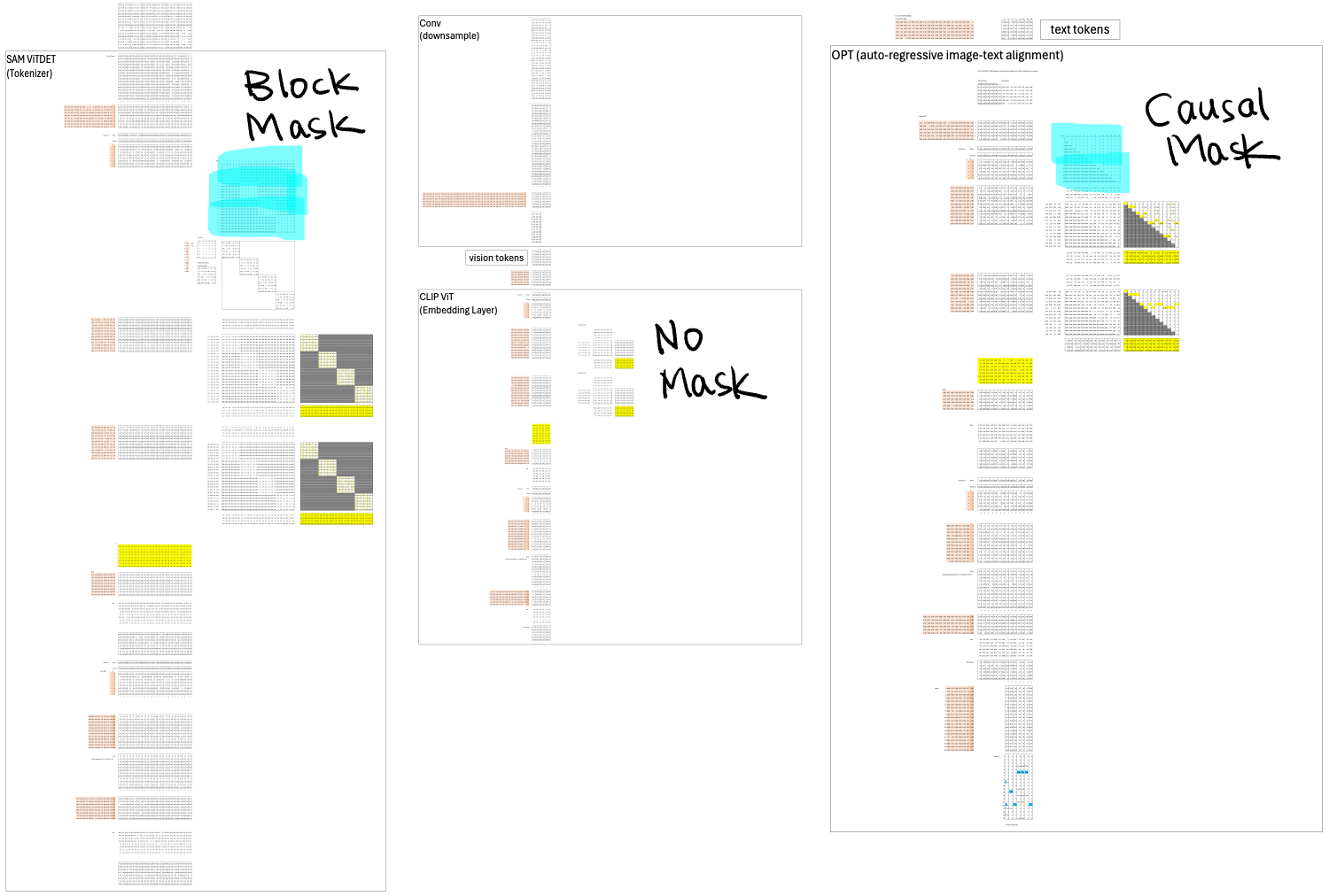
Now that we’ve seen how each layer contributes to the overall pipeline, it’s worth looking at how their attention mechanisms differ. Each of the three Transformers—SAM ViTDeT, CLIP ViT, and OPT—uses a distinct masking strategy, reflecting the kind of information it needs to capture.

SAM ViTDeT is responsible for extracting local features. It uses block-based attention, meaning each token can only attend to others within its local block. This restriction helps the model focus on fine-grained visual patterns without being distracted by distant regions.

CLIP ViT, on the other hand, combines those local features into global representations. To do this, it needs full attention, allowing every token to see every other token. No mask is used here. However, global attention is computationally expensive, so CLIP ViT can handle far fewer tokens. That’s one reason we introduced the convolution layer earlier—to reduce 24 local tokens into 6 global ones before feeding them into CLIP ViT.

Finally, OPT is responsible for autoregressive decoding to align the visual and text modalities. It uses a causal mask, meaning each new query token can only attend to itself and the tokens that came before it—not the ones that come after. This is what enforces the left-to-right generation process, ensuring the model learns to predict the next word step by step, just like a language model.

Position Embeddings

Just like attention masks, each Transformer in the DeepSeek OCR stack handles positional information differently. Position embeddings tell the model where each token is located—whether in an image grid or a text sequence—and each layer encodes that spatial or sequential structure in its own way.

CLIP ViT and OPT both use learnable positional embeddings. Instead of relying on the fixed sine and cosine patterns from the original Transformer paper, they treat position as a set of trainable parameters. This allows the model to adaptively learn positional relationships from data rather than being constrained by a hardcoded formula. At the time these models were designed, RoPE (Rotary Positional Embedding) had not yet become the standard choice, so learnable embeddings were the preferred method.

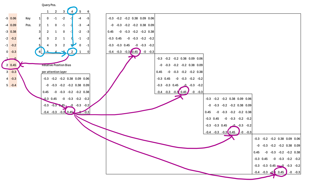
SAM ViTDeT, however, takes a different approach. Since it only needs to reason about positions within each local block, it uses relative position embeddings. This means the model doesn’t care about absolute coordinates—it only learns how far one token is from another inside the same attention window.

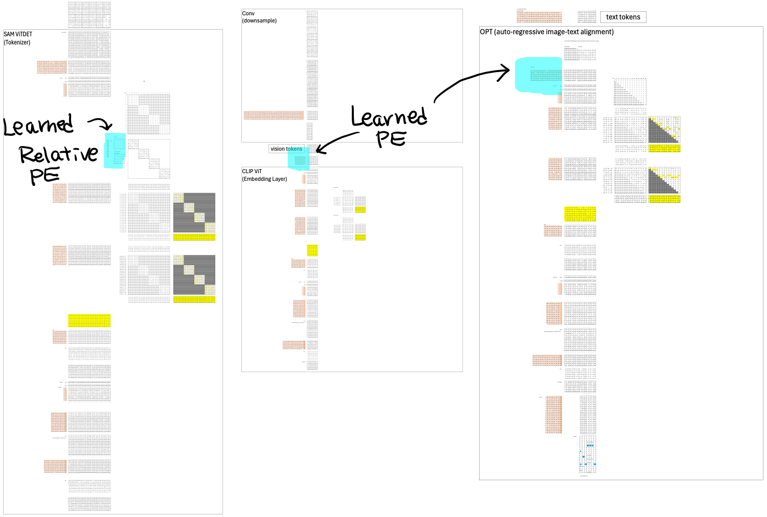
To see how this works, consider a 6×6 attention block. Each query token can be at most 5 positions ahead (+5) or 5 positions behind (–5) of a key token. That gives us 11 possible relative offsets, ranging from –5 to +5. The model learns one weight for each of these 11 relative positions, effectively capturing how attention should shift based on relative distance rather than absolute location.

Layer Normalization

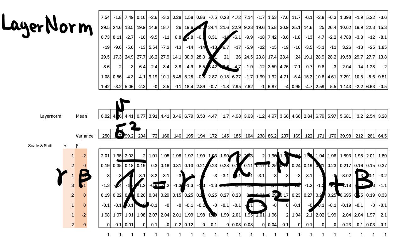
All three models—SAM ViTDeT, CLIP ViT, and OPT—use Layer Normalization to stabilize training and keep activations within a manageable range. Around 2023, LayerNorm was still the standard choice across most Transformer architectures; RMSNorm had not yet become mainstream.

Below I wrote the fomulas on top of one of the LayerNorm block.

This article is getting long—but I really enjoyed putting it together.

I know I’ve answered a lot of questions, but I’ve probably opened up even more along the way. There’s no way to cover everything here, so I’ll stop before it turns into a full lecture.

If something sparked your curiosity, or you’d like me to go deeper on a specific part, drop your questions in the comments—I’d love to continue the discussion there.

Download

This Frontier AI Excel Blueprints are available to AI by Hand Academy members. You can become a member via a paid Substack subscription.