Einsum Blueprint: Part 1 - Outer Product to GQA

Frontier Model Math by hand ✍️

(P.S. This issue is written for advanced AI engineers and researchers. It is part of the premium Frontier subscription. If you are a beginner, please check out my free Foundation series, lectures, walkthroughs, and Excel exercises.)

Who is the other Nobel Prize winner whose work quietly powers frontier AI research?

Albert Einstein—the physicist who introduced the Einstein summation convention (einsum).

His notation, created over a century ago to simplify tensor equations in physics, is now used intensively in frontier AI labs and open-source implementations around the world to express the core computations behind modern neural networks.

Therefore, not being able to read or write einsum is a form of illiteracy in frontier AI research.

For example, Albert Gu’s Mamba open-source implementation uses einsum extensively. And by the way, if you’ve ever spoken with Albert and were struck by his intelligence like I was, you may wonder who he was named after. When reading his code, for instance, I had trouble reading this line:

y = torch.einsum(”bhpn,bn->bhp”, ssm_state.to(dtype), C)

Another example, when I studied Grouped Query Attention from Google Research, I encountered this in the source code:

similarity = einsum(query, key, “b g h n d, b h s d -> b g h n s”)

I felt “illiterate” myself—until I spent considerable time and effort learning how einsum really works.

Over the past few months, I have been building this Blueprint to share the approach and insights that helped me master einsum, so others can bridge the same gap between math, code, and intuition.

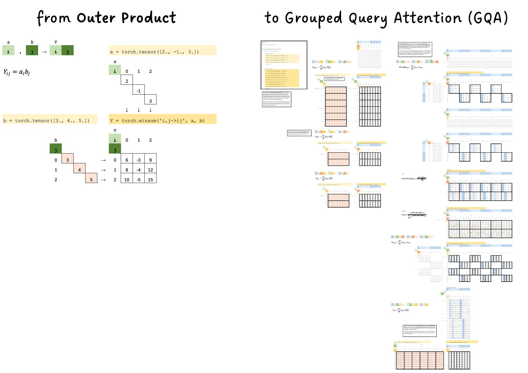
In Part 1, I’ll take you from the most basic concept—the outer product—and incrementally build up to Grouped Query Attention (GQA).

If this Blueprint proves helpful, I plan to create Part 2, where we’ll extend these ideas to Mamba and one of the latest linear transformer variants.

Table of Content

1. How to Use this Blueprint?

2. Outer Product

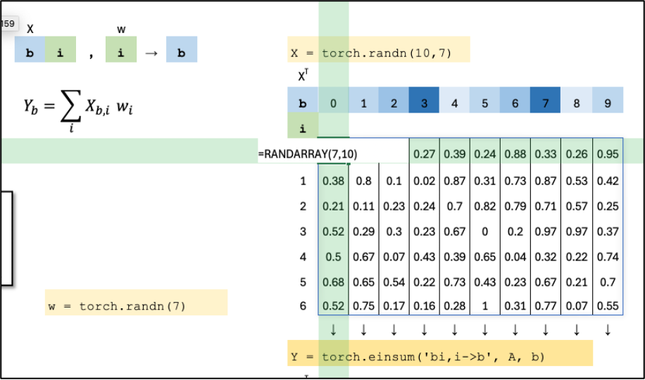
3. Scaled Sum

4. Dot Product

5. Dot Product (Batch)

6. Matrix Multiplication

   1. Increase the input dimension (k)

   2. Increase the output dimension (n)

7. Matrix Multiplication (Batch)

   1. Increase the input dimension (k)

   2. Increase the output dimension (n)

8. Linear Layer

9. Linear Layer (Batch)

10. Linear Layer (Batch x Time)

11. Single Head Attention (Single Sample)

12. Single Head Attention (Batch)

13. Multi-Head Attention (MHA)

14. Grouped Query Attention (GQA)

How to Use this Blueprint?

Select a cell. Press [F2] to view the underlying formula.

Select a line. Use “Formulas > Trace Dependents” to see the corresponding tensor and tensor operations

Select an index in an Einsum expression. Use “Formulas > Trace Dependents” to see the corresponding index in the math view

Outer Product

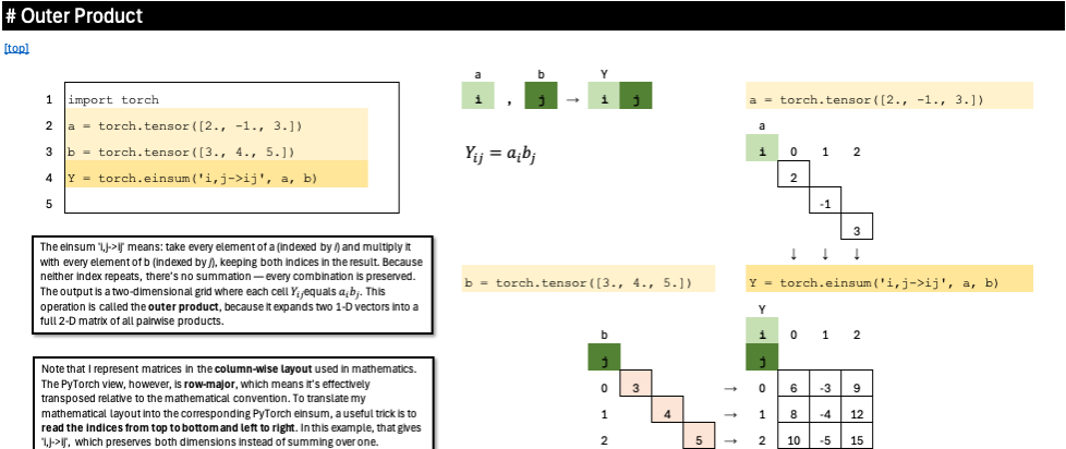
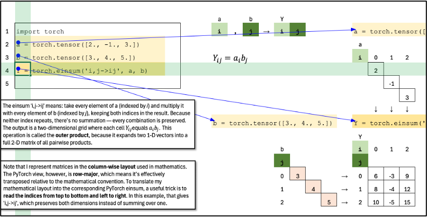
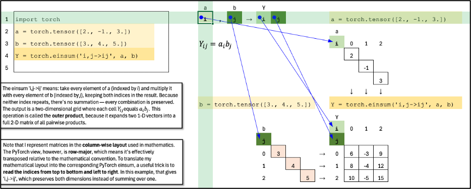
The einsum ‘i,j->ij’ means: take every element of a (indexed by i) and multiply it with every element of b (indexed by j), keeping both indices in the result. Because neither index repeats, there’s no summation — every combination is preserved. The output is a two-dimensional grid where each cell Y_ij equals a_i b_j. This operation is called the outer product, because it expands two 1-D vectors into a full 2-D matrix of all pairwise products.

Dot Product

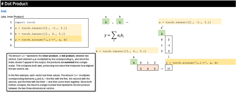
The einsum ‘i,i->’ represents the inner product, or dot product, between two vectors. Each element a_i is multiplied by the corresponding b_i, and since the index i doesn’t appear in the output, the products are summed into a single scalar. This collapses both axes, producing one value that measures how aligned the two vectors are.

Linear Layer (Batch)

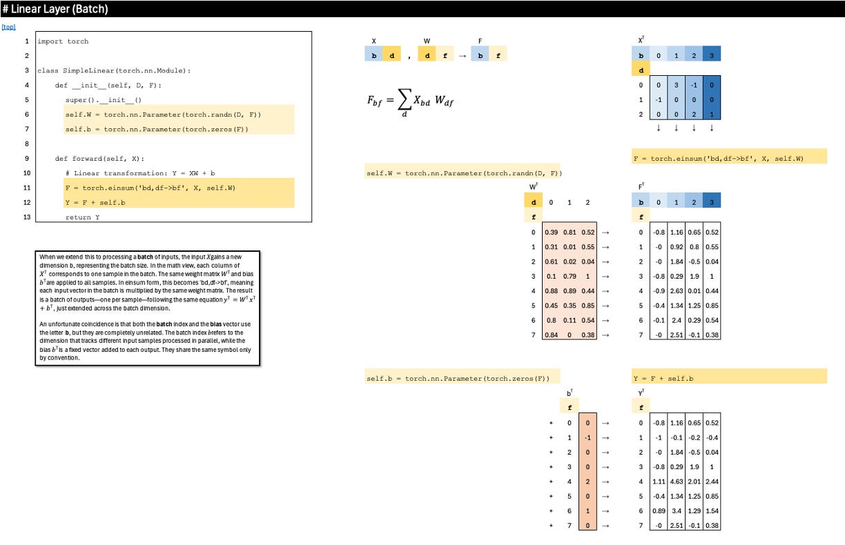
When we extend this to processing a batch of inputs, the input X gains a new dimension b, representing the batch size. In the math view, each column of X^T corresponds to one sample in the batch. The same weight matrix W^T and bias b^T are applied to all samples. In einsum form, this becomes ‘bd,df->bf’, meaning each input vector in the batch is multiplied by the same weight matrix. The result is a batch of outputs—one per sample—following the same equation y^T=W^T x^T+b^T, just extended across the batch dimension.

⬇️ Download the Blueprint below to study the rest (for Frontier Subscribers only)