
LinearLayer+LoRA: PyTorch, BLAS, CUDA
Frontier AI Excel Blueprint

This paid post is currently open for free preview
Why is it so confusing for people to understand something as simple as a linear layer — even for AI engineers who work in top AI labs? There are three main sources of confusion that make it hard for AI engineers to bridge the gap between math and implementation.
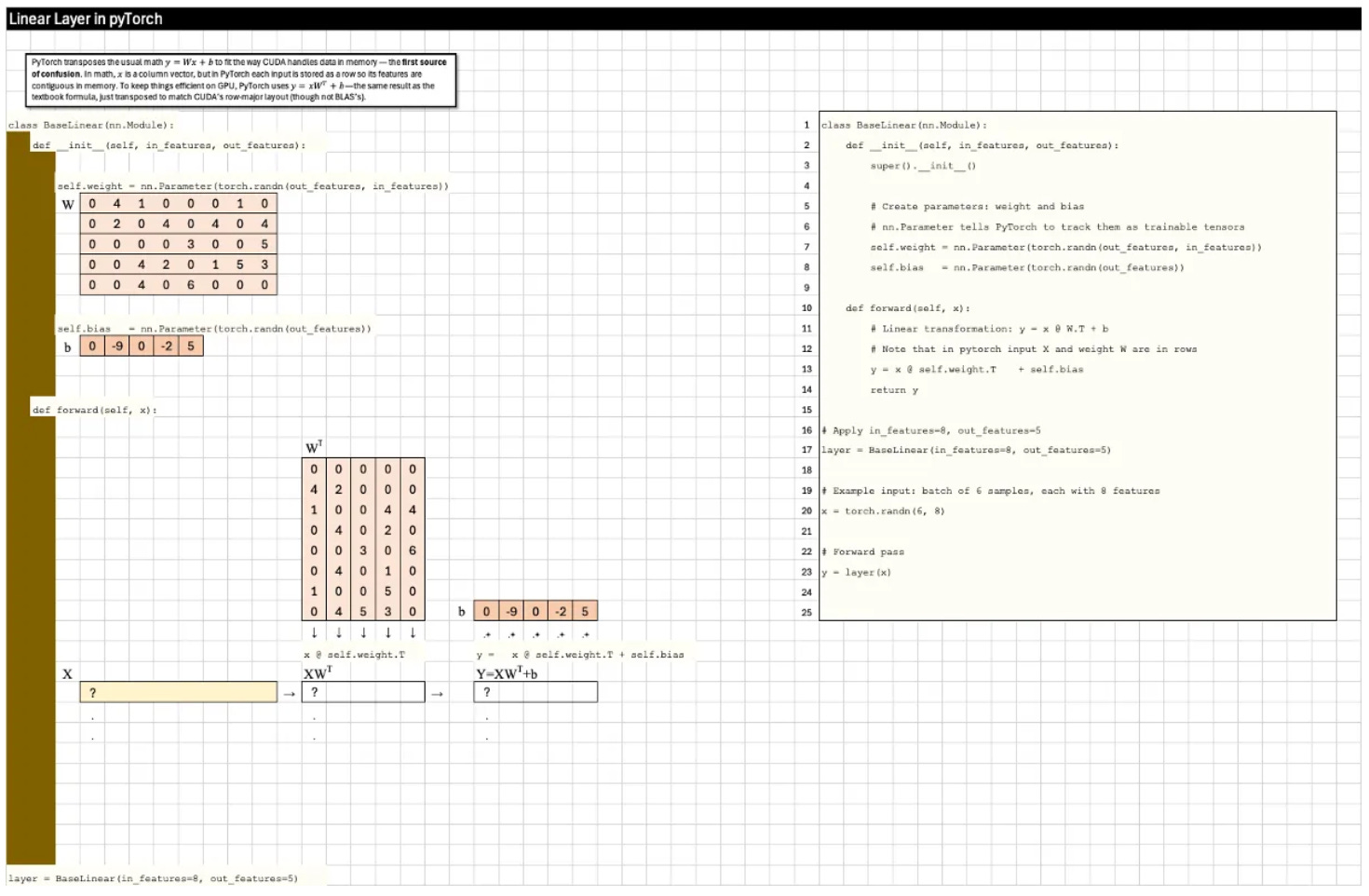
First, PyTorch transposes the math y=Wx+b to y=xW^T+b to match CUDA’s row-major layout.
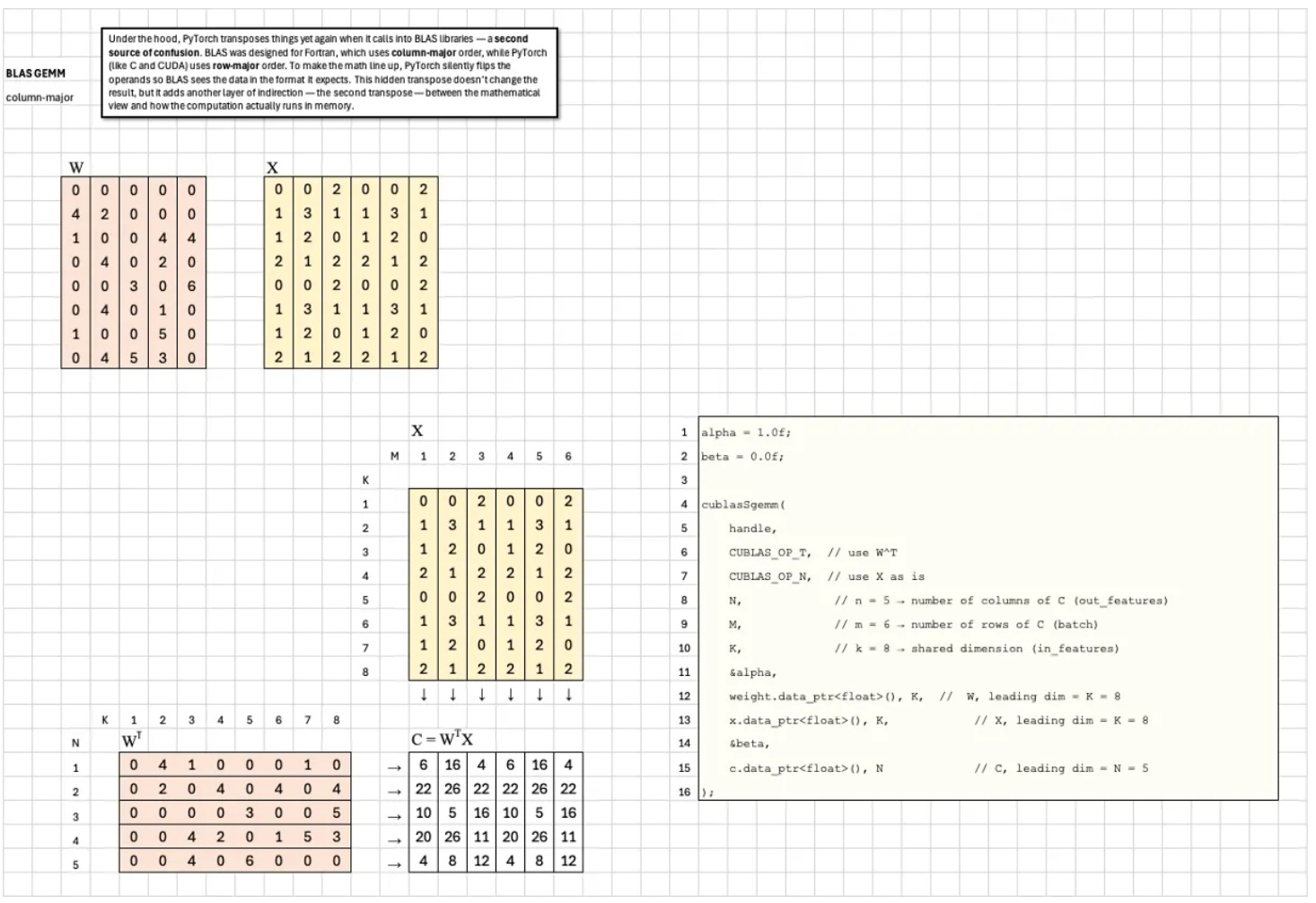
Second, it transposes again for BLAS, which uses column-major order.
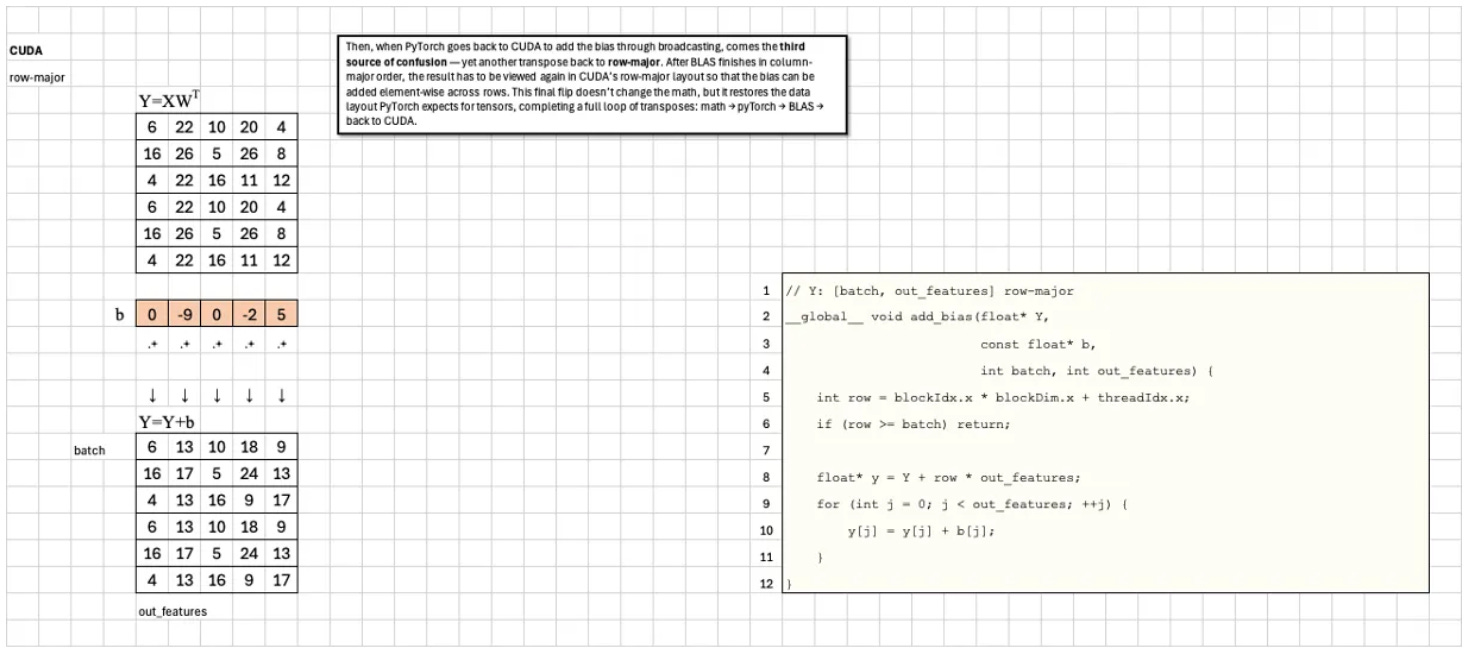
Third, it transposes back to row-major when adding the bias.
All three produce the same result but hide the simple math behind layers of memory optimization.
Let’s clear this confusion once for all!
In the AI by Hand ✍️ view, everything starts with the math. A linear layer is just a matrix where rows are weights (one per output unit) and columns are feature vectors (one per instance). When you multiply them, each cell in the output naturally represents the intersection between a weight row and a feature column. The shape of the output pops out visually: the number of rows equals the number of outputs, and the number of columns equals the batch size (or feature instances).
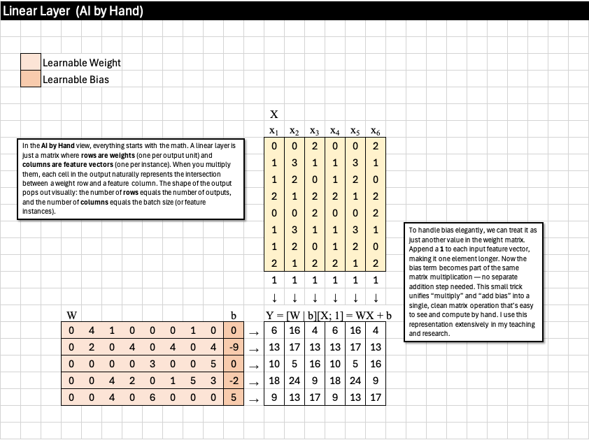
To handle bias elegantly, we can treat it as just another value in the weight matrix. Append a 1 to each input feature vector, making it one element longer. Now the bias term becomes part of the same matrix multiplication — no separate addition step needed. This small trick unifies “multiply” and “add bias” into a single, clean matrix operation that’s easy to see and compute by hand. I use this representation extensively in my teaching and research.
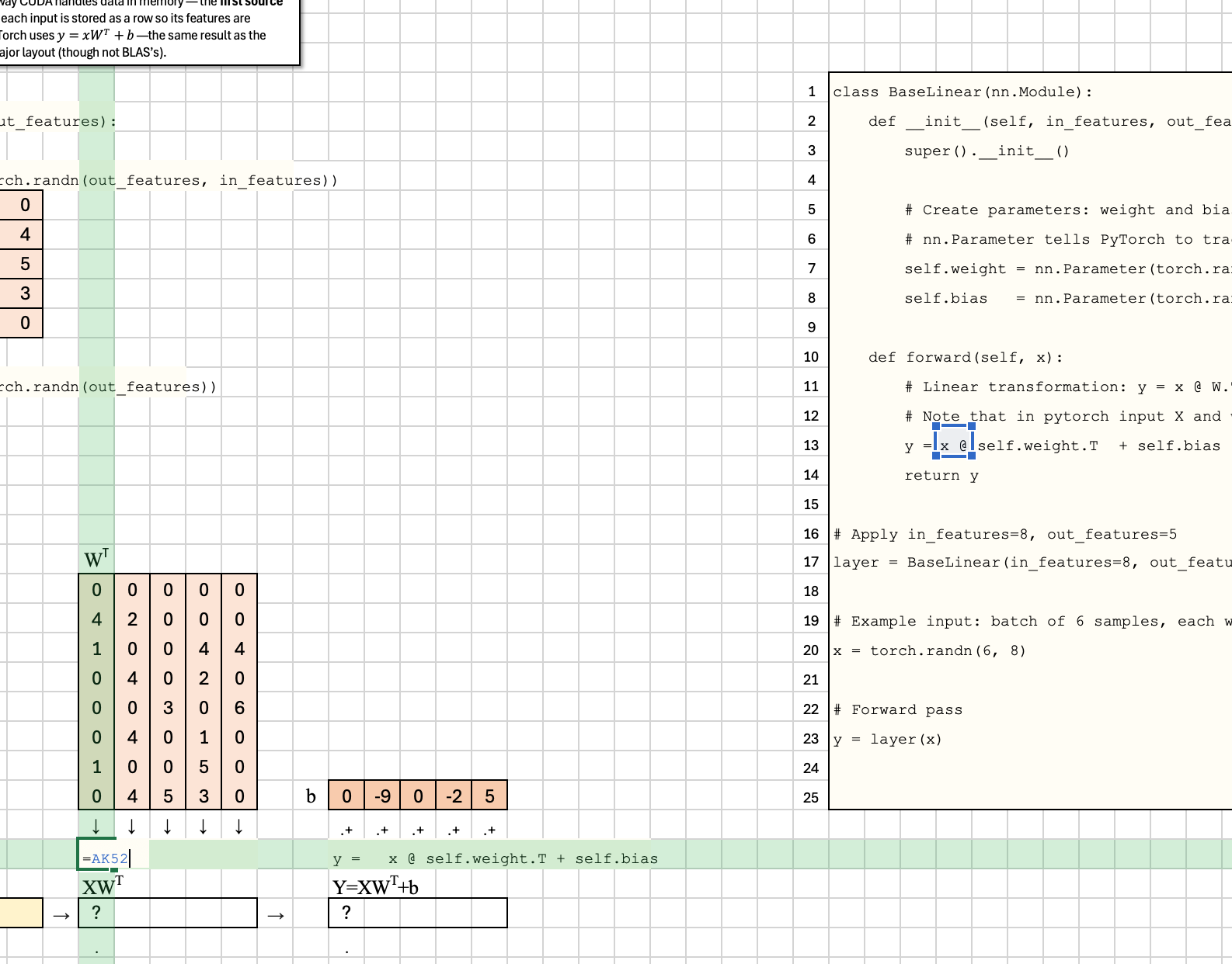
PyTorch transposes the usual math y=Wx+b to fit the way CUDA handles data in memory — the first source of confusion. In math, x is a column vector, but in PyTorch each input is stored as a row so its features are contiguous in memory. To keep things efficient on GPU, PyTorch uses y=xW^T+b— the same result as the textbook formula, just transposed to match CUDA’s row-major layout (though not BLAS’s).
👇 Scroll to the bottom to download this Excel Blueprint. Tip: Press F2 to highlight which line of PyTorch code a calculation corresponds to.
Under the hood, PyTorch transposes things yet again when it calls into BLAS libraries — a second source of confusion. BLAS was designed for Fortran, which uses column-major order, while PyTorch (like C and CUDA) uses row-major order. To make the math line up, PyTorch silently flips the operands so BLAS sees the data in the format it expects. This hidden transpose doesn’t change the result, but it adds another layer of indirection — the second transpose — between the mathematical view and how the computation actually runs in memory.
Then, when PyTorch goes back to CUDA to add the bias through broadcasting, comes the third source of confusion — yet another transpose back to row-major. After BLAS finishes in column-major order, the result has to be viewed again in CUDA’s row-major layout so that the bias can be added element-wise across rows. This final flip doesn’t change the math, but it restores the data layout PyTorch expects for tensors, completing a full loop of transposes: math → PyTorch → BLAS → CUDA → PyTorch.
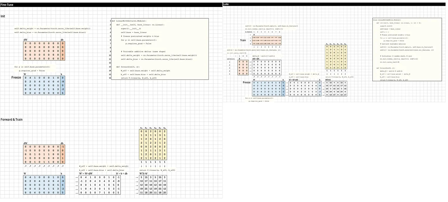
Finally, you have all you need to follow the “Math-PyTorch” Blueprint I made for Fine-tuning vs LoRA. 🙌
Download
This Frontier AI Excel Blueprints are available to AI by Hand Academy members. You can become a member via a paid Substack subscription.
Adding the PyTorch and CUDA, adds an additional dimension of clarity.