SwiGLU
Activation series · 12 of 12
Activation › SwiGLU
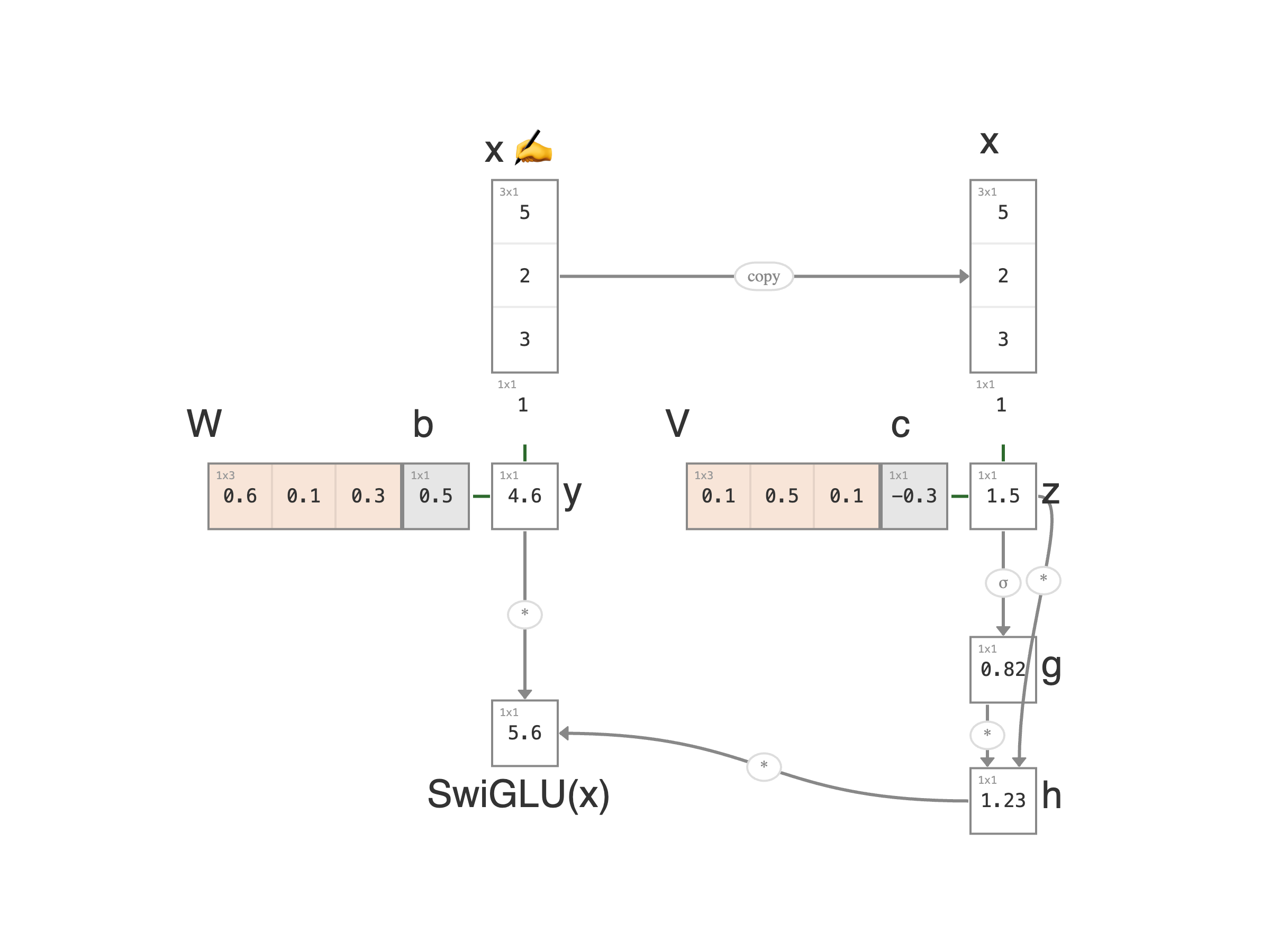
SwiGLU is GLU with the sigmoid gate replaced by a SiLU gate. The two-branch shape is identical; the only change is that the gate is no longer capped at 1 — it can push past full rated capacity into overdrive.
Typhoon Aftermath (4 of 4)
Let's imagine an extreme typhoon, one of those once-in-a-decade storms. The GLU-style controller is doing its job: the sigmoid gate has already saturated near 1, full rated pump capacity, nothing more. But the water keeps rising. The pumps are doing everything they're "allowed" to do, and the streets are still flooding.
What if we override the safety limit? The new controller is no longer capped at 1. At low pressure it behaves like a sigmoid, mildly engaging the pump. At high pressure it keeps responding linearly with the input, past the safety limit, into overdrive. That's SiLU as a gate (gate value = b · σ(b)) instead of plain sigmoid.
That's SwiGLU. Same two-branch GLU structure: one linear branch becomes the value, one linear branch becomes the gate, multiply elementwise. The only change is the gate's activation function: SiLU instead of σ. The gate can now amplify, not just attenuate.
Why the deep-learning world cares: every frontier large language model uses SwiGLU in its feed-forward blocks. A pump that can push past its rated max produces measurably better gradients than one capped at 100%. In the deep stacks of transformer layers where each layer's output feeds the next, an unbounded gate keeps the signal alive layer after layer.
Walking through the Math
1. Input: a feature vector `x = (5, 2, 3)` (same setup as GLU). Append a 1 at the bottom for the bias trick.
2. Severity (left branch): y = Wx + b = 0.6 × 5 + 0.1 × 2 + 0.3 × 3 + 0.5 × 1 = 4.6, identical to GLU's severity branch.
3. Gate input (right branch): z = Vx + c = 0.1 × 5 + 0.5 × 2 + 0.1 × 3 + (-0.3) × 1 = 1.5, same as GLU.
4. Sigmoid: g = σ(z) = σ(1.5) ≈ 0.82, same as GLU. This number is bounded between 0 and 1.
5. SiLU (new step): h = z × g = 1.5 × 0.82 ≈ 1.23. Multiply the sigmoid result by z. This is what makes the gate unbounded above, because z itself isn't bounded.
6. Multiply: o = y × h = 4.6 × 1.23 ≈ 5.7. The SwiGLU output.
The only change from GLU is step 5: a single extra multiplication. That one operation transforms a saturating gate (σ ≤ 1) into an amplifying one. At z = 1.5 the gate is already 1.23, past GLU's ceiling of 1; at z = 3 it would be near 2.86, almost three times the ceiling.
Reading the Numbers
Same setup as GLU: each storm is a feature vector `x = (rainfall, tide, wind)`, the value branch produces a severity, the gate branch produces a pump-power signal, and the elementwise product is the water actually pushed back over the levy. The only change is that the gate is SiLU instead of sigmoid, no longer capped at 1.
The gate at `(5, 2, 3)` already pushes past 1 (that's overdrive), and at `(8, 4, 5)` it's running at over 3× rated capacity. A sigmoid-gated GLU controller, on the same severities, would have produced gate values of 0.67, 0.86, 0.96: capped near 1, saturating fast, no extra response left for the most extreme storm. SwiGLU keeps amplifying when GLU has already given up.
Diving into Equations
The pump-station equation in this article shows the SwiGLU activation in isolation. The form modern LLMs actually use wraps SwiGLU into a feed-forward block with three weight matrices, named for what they do:
`W_gate` projects the input up to the hidden dimension and feeds the gate; `W_up` does the same projection for the value branch; `W_down` projects the gated result back down to the model dimension.
Compare to the older ReLU feed-forward block, with just two (one up, one down):
The extra matrix is the cost of having a separate value branch and gate branch. To keep the parameter count comparable, every modern frontier transformer shrinks the inner ("hidden") dimension of the SwiGLU block to about two-thirds of what the equivalent ReLU block uses, a slightly narrower hidden layer in exchange for the gating expressiveness.
This is the equation you'll find in frontier-model source code, where the matrices are typically named `gate_proj`, `up_proj`, and `down_proj`.
← Previous:
GLU


