SwiGLU: The Activation Function Behind Frontier AI

Essential AI Math Excel Blueprints

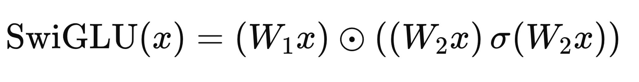
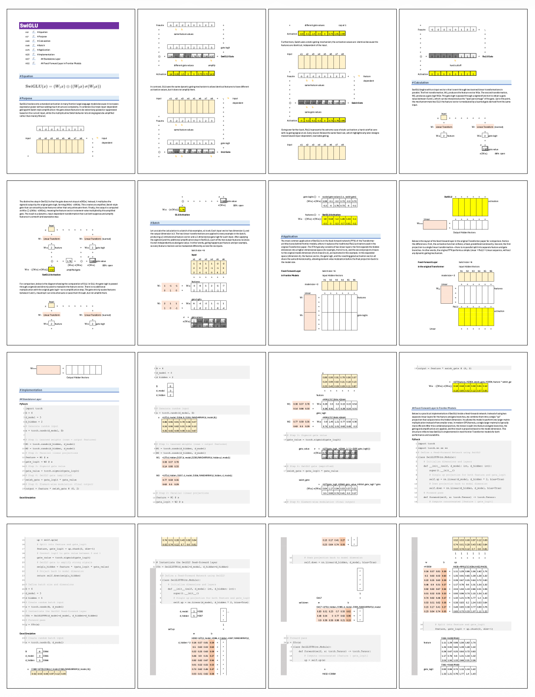
SwiGLU has become a standard activation in many frontier large language models because it increases expressive power without adding much structural complexity. It combines GLU-style input-dependent gating with Swish-style amplification: the gate allows features to be selectively passed or suppressed based on the current input, while the multiplicative Swish behavior lets strong signals be amplified rather than merely filtered.

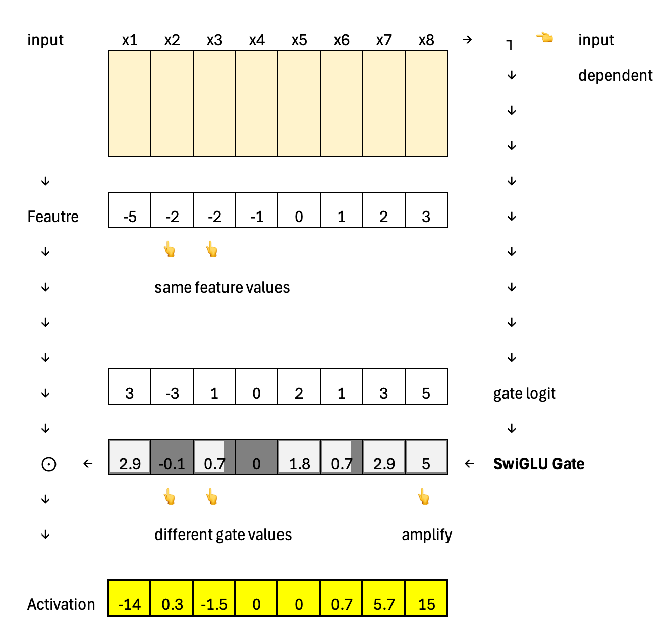
In contrast, GLU uses the same dynamic gating mechanism to allow identical features to have different activation values, but it does not amplify them.

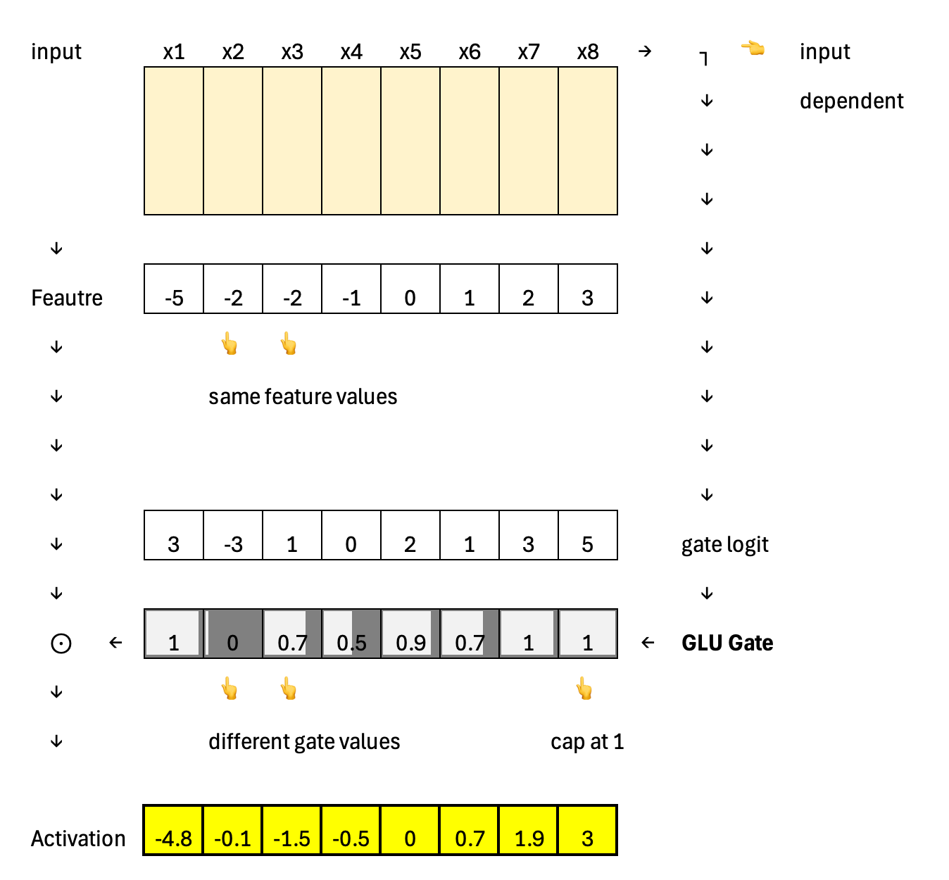
Furthermore, Swish uses a static gating mechanism; the activation values are identical because the features are identical, independent of the input.

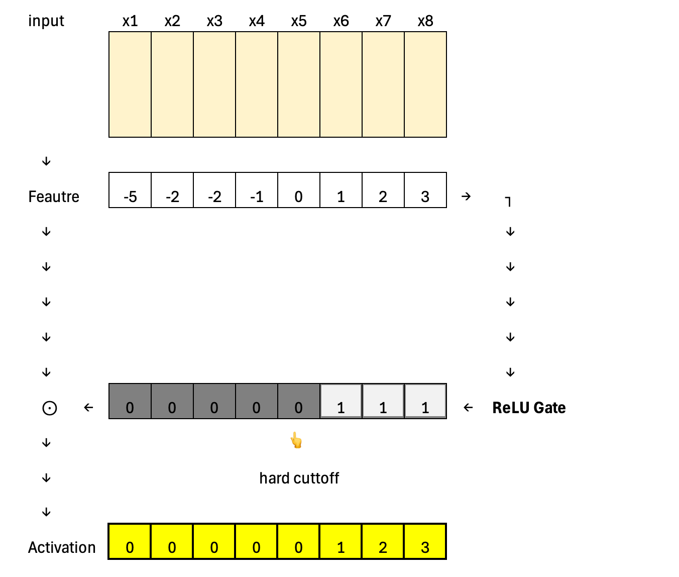
Going even further back, ReLU represents the extreme case of static activation: a hard cutoff at zero with no gating signal at all. Every neuron follows the same fixed rule, which highlights why later designs moved toward input-dependent, learnable gating.

Calculation

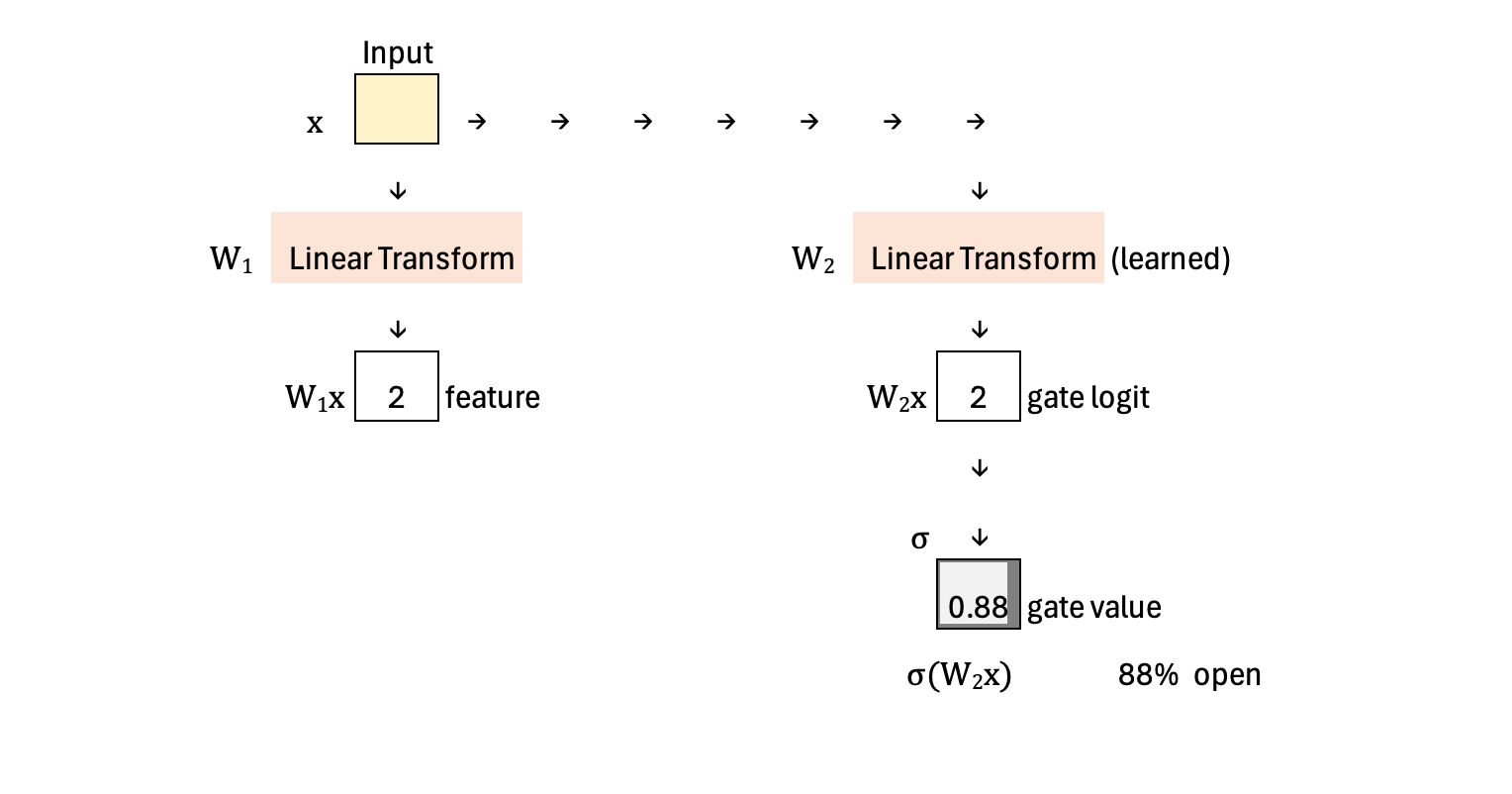
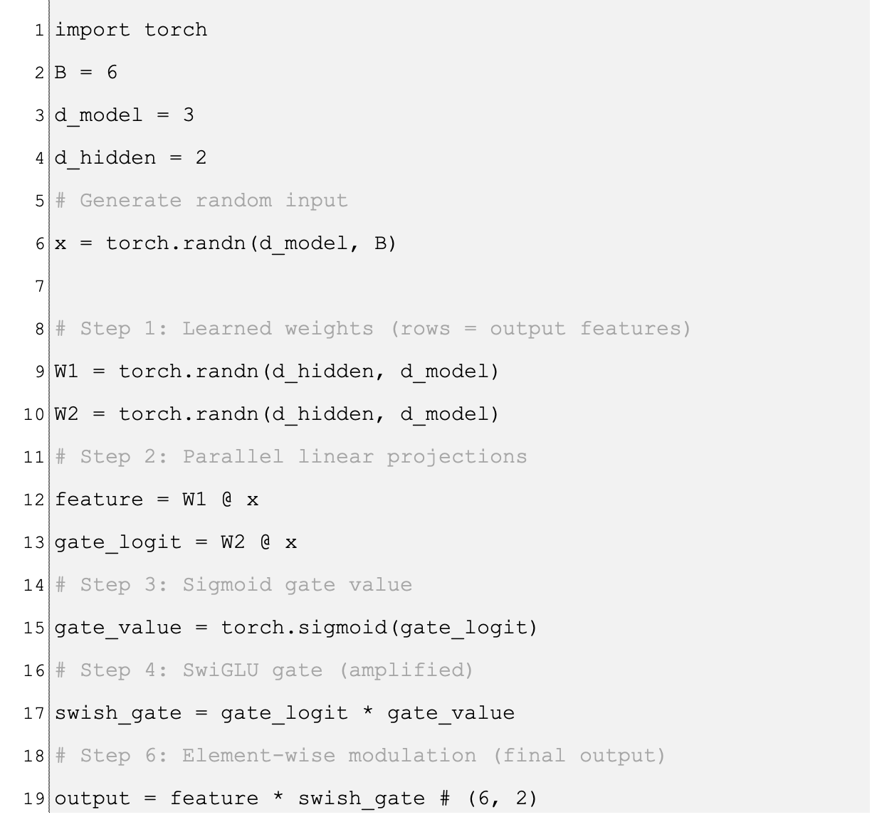
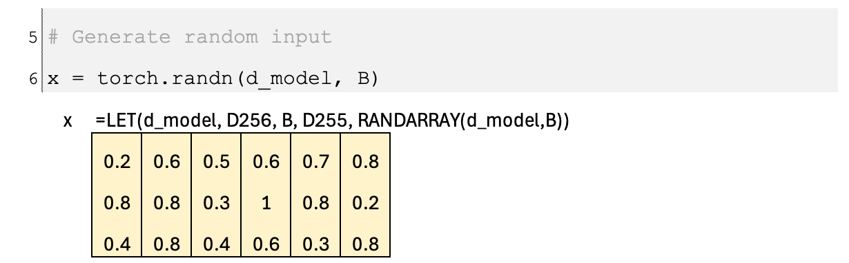
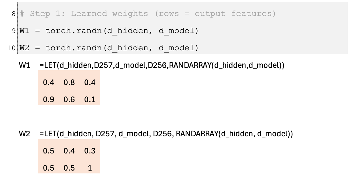
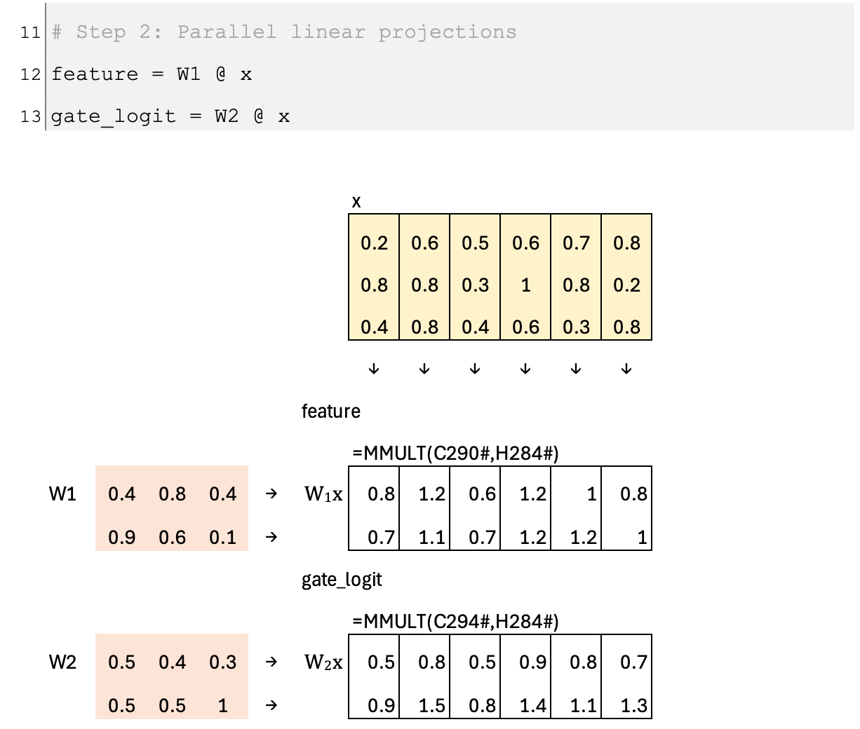
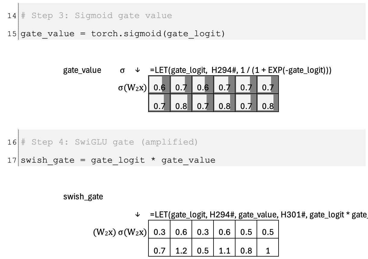
SwiGLU begins with an input vector x that is sent through two learned linear transformations in parallel. The first transformation, W1, produces the feature vector W1x. The second transformation, W2, produces a gate logit W2x. This gate logit is passed through a sigmoid function to obtain a gate value between 0 and 1, which can be interpreted as the “open percentage” of the gate. Up to this point, the mechanism matches GLU: the feature vector is modulated by a learned gate derived from the same input.

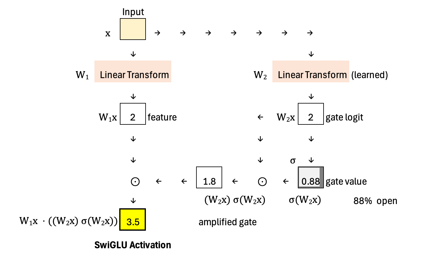
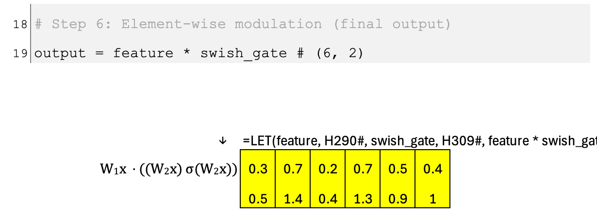
The distinctive step in SwiGLU is that the gate does not stop at σ(W2x). Instead, it multiplies the sigmoid output by the original gate logit, forming (W2x) · σ(W2x). This creates an amplified, Swish-style gate that can smoothly scale features rather than only attenuate them. Finally, the output is computed as W1x ⊙ ((W2x) · σ(W2x)), meaning the feature vector is element-wise multiplied by this amplified gate. The result is a dynamic, input-dependent transformation that can both suppress and amplify features in a smooth and expressive way.

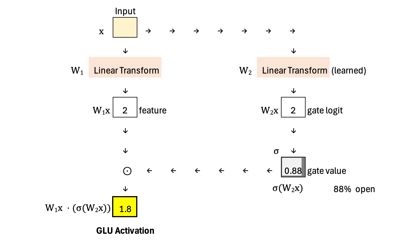
For comparison, below is the diagram showing the computation of GLU. In GLU, the gate logit is passed through a sigmoid and directly used to modulate the feature vector. There is no additional multiplication with the original gate logit—so no amplification step. The gate strictly scales features between 0 and 1, meaning it can only attenuate or pass them through, but not amplify them.

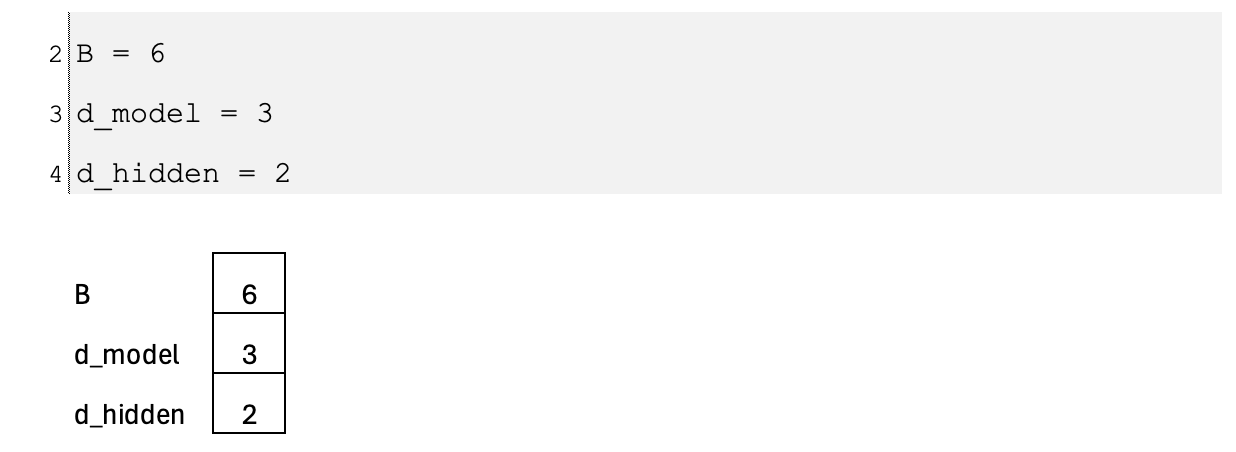
Batch

Let us scale the calculation to a batch of six examples, x1 to x6. Each input vector has dimension 3, and the output dimension is 2. The two linear transformations are applied to every example in the batch, producing a 2-dimensional feature vector and a 2-dimensional gate logit for each input. After applying the sigmoid (and the additional amplification step in SwiGLU), each of the two output features receives its own independently scaled gate value. In other words, gating happens per feature and per example, so every feature channel can be modulated differently across the six inputs.

Application

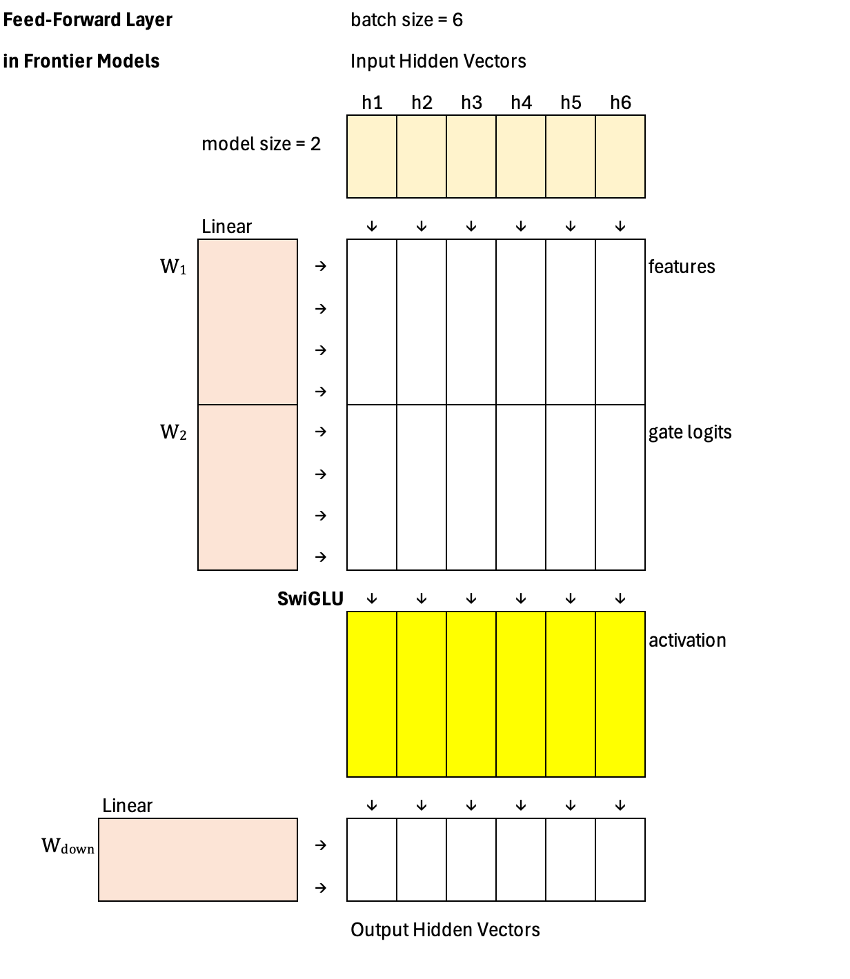
The most common application of SwiGLU is in the feed-forward network (FFN) of the Transformer architectures behind frontier models, where it replaces the traditional ReLU activation used in the original Transformer paper. The FFN typically consists of two linear layers: the first expands the hidden dimension into a higher-dimensional space (for example, from 2 to 4), and the second projects it back to the original model dimension (from 4 back to 2), as illustrated in this example. In this expanded space (dimension 4), the feature vector, the gate logit, and the resulting gated activation vector all share the same dimensionality, allowing element-wise modulation before the final projection back to the model size.

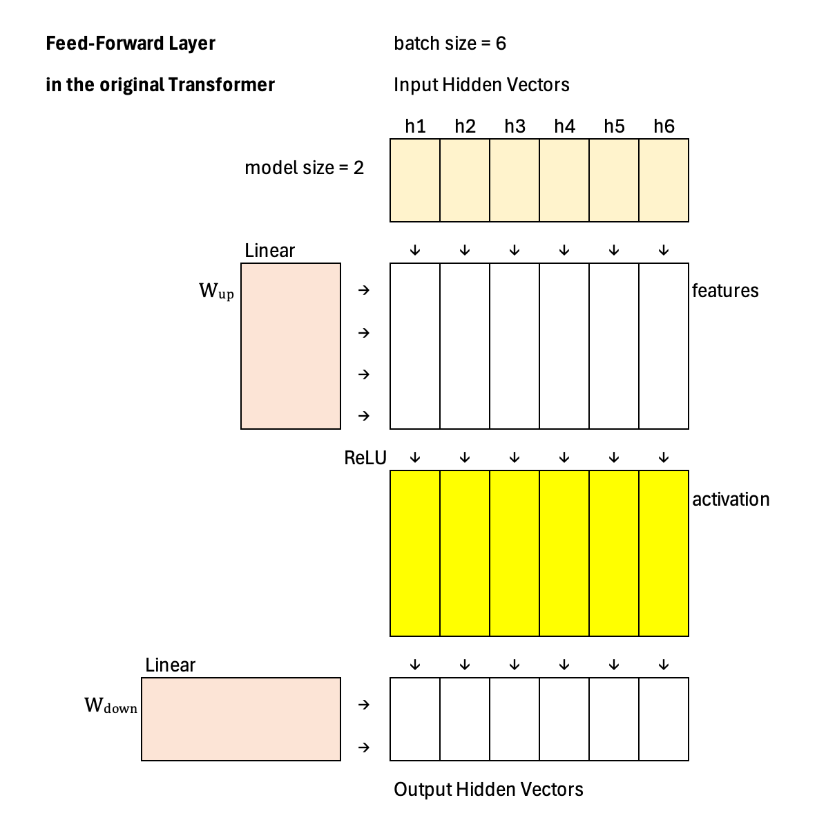
Below is the layout of the feed-forward layer in the original Transformer paper for comparison. Notice the differences. First, the activation function is ReLU, a fixed, predefined nonlinearity. Second, the first projection is a single linear transformation—there is no parallel split into separate feature and gate branches. In other words, the original FFN performs a simple Linear → ReLU → Linear sequence, without any dynamic gating mechanism.

Implementation: Standalone Layer

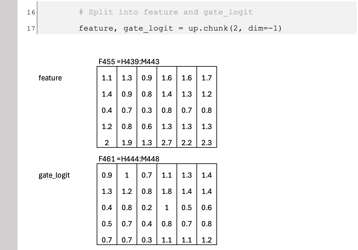
PyTorch

---

Excel Emulation

Implementation: Feed-Forward Layer in Frontier Models

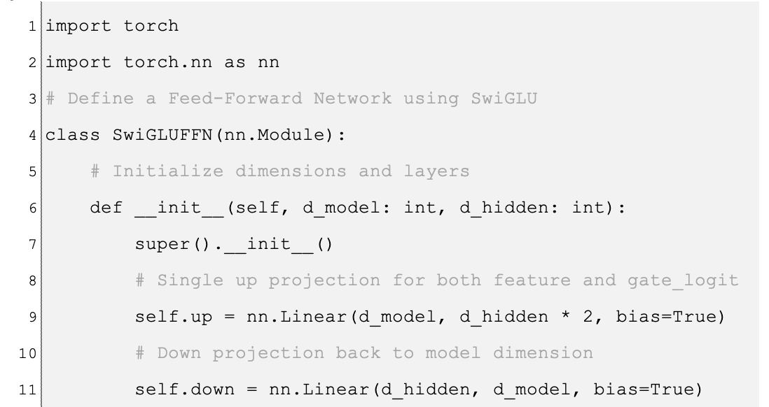
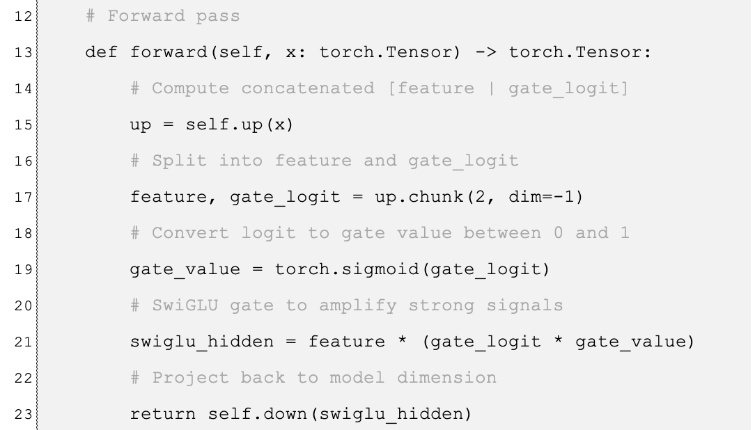
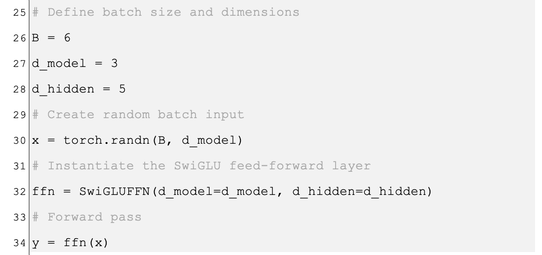
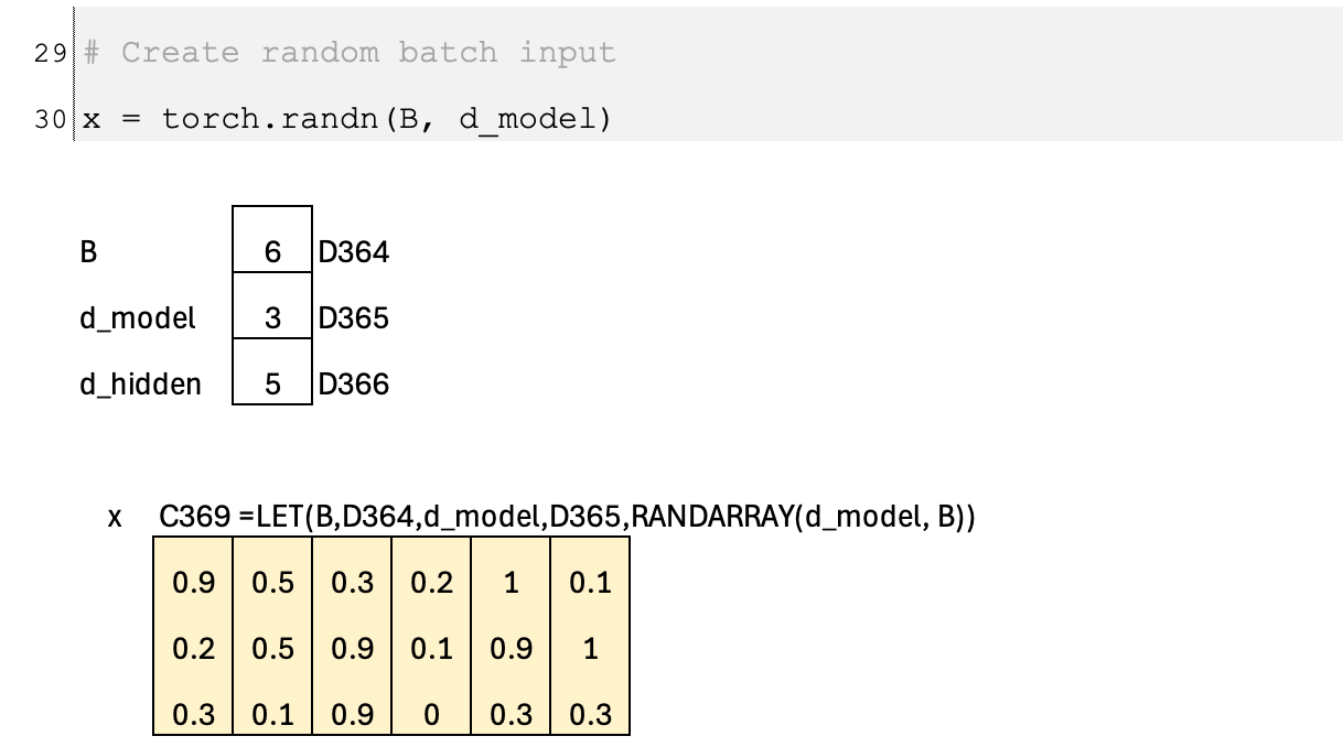
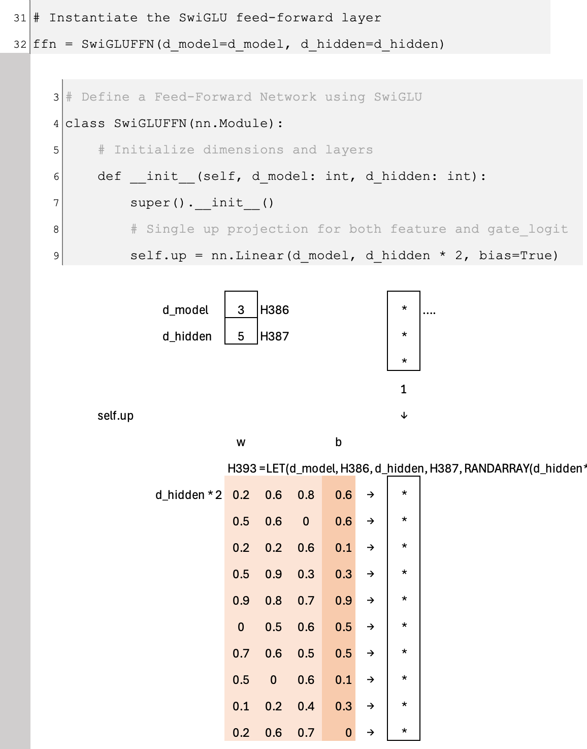
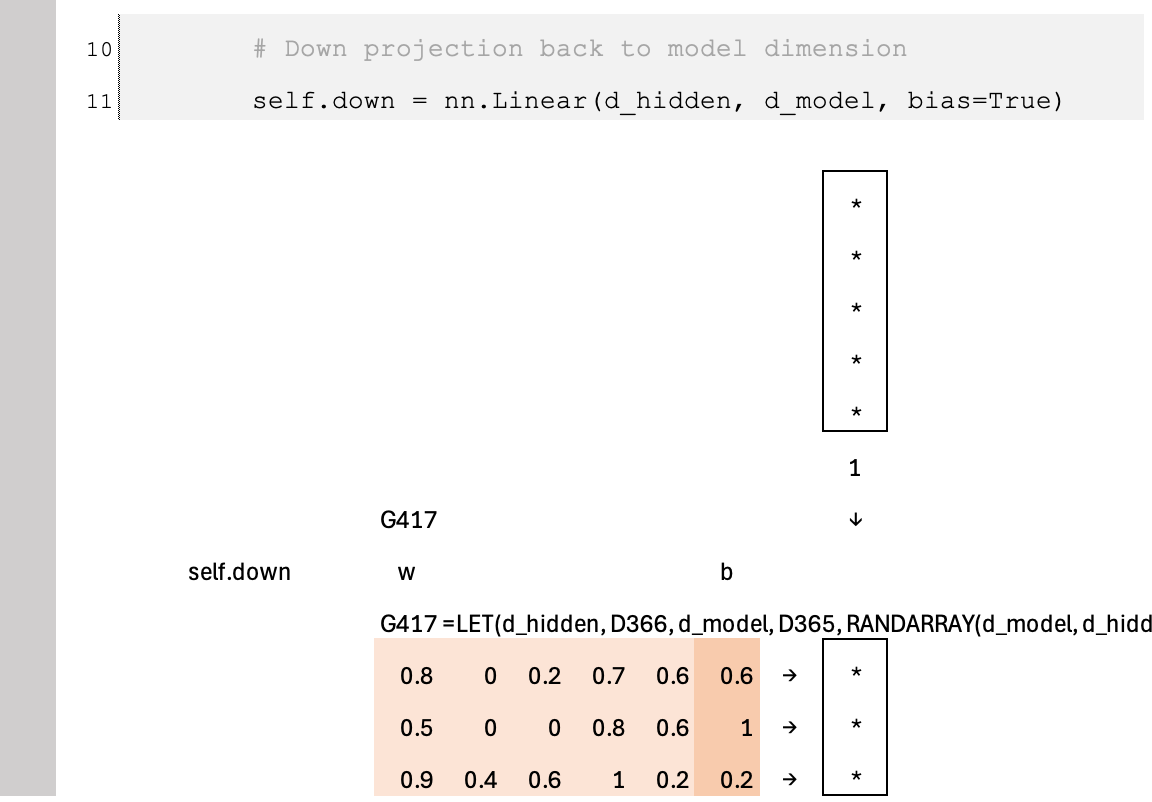
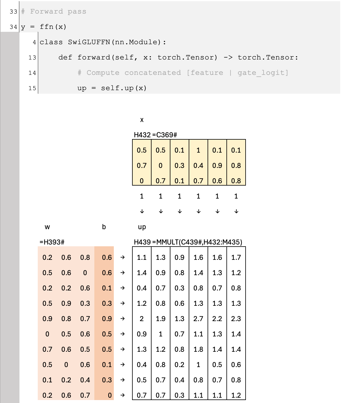
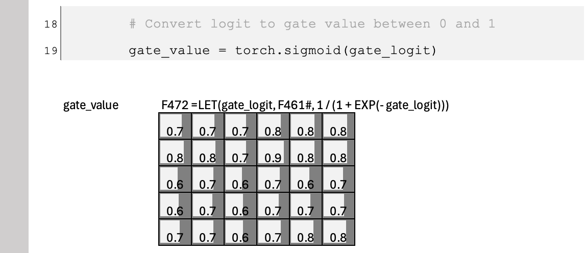
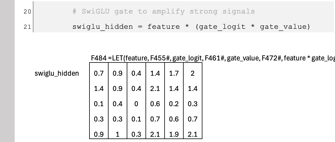
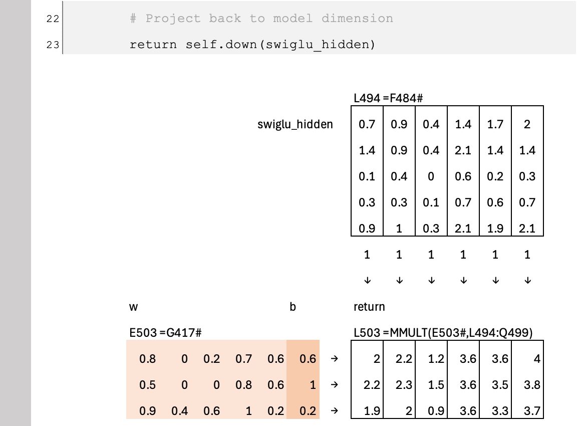
Below is a practical implementation of SwiGLU inside a feed-forward network. Instead of using two separate linear layers for the feature and gate branches, we combine them into a single “up” projection that outputs twice the hidden dimension. his allows the model to perform one larger matrix multiplication instead of two smaller ones. In modern GPU kernels, a single larger matmul is typically more efficient After this combined projection, the tensor is split into feature and gate branches, the gating and amplification are applied, and the result is projected back to the model dimension. This structure reflects how SwiGLU is implemented in most frontier Transformer models for both performance and scalability.

PyTorch

Excel Emulation

Excel Blueprint

🔗 View the Excel Blueprint Online

(Limited time preview)

This is part of the Essential AI Math Blueprints series. Get the full series by joining the AI by Hand Academy.