
Pretrain vs Fine-Tune
Fine-Tuning series: 2 of 8

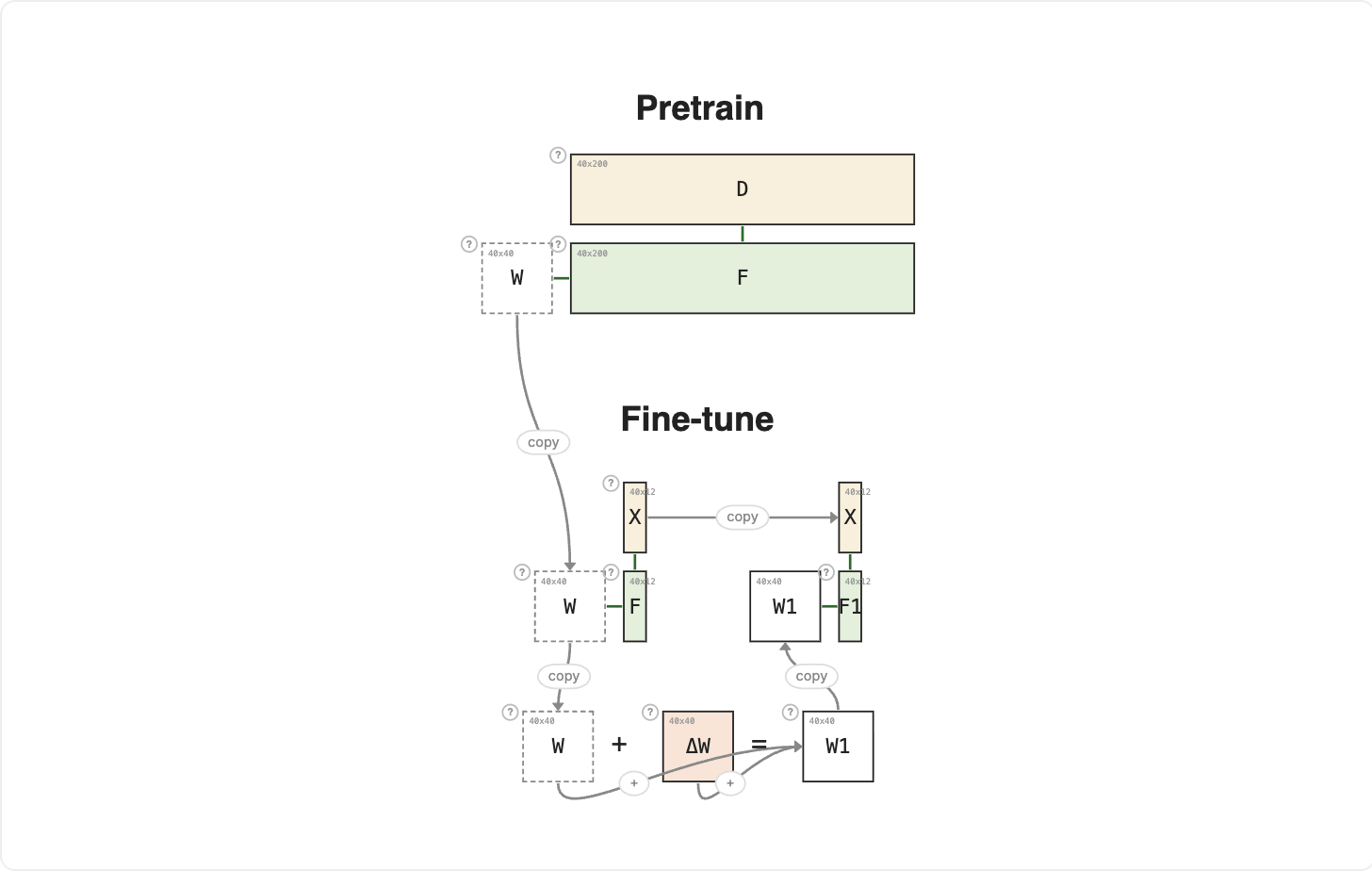
The previous lesson showed W + ΔW = W₁ as a single abstract step. That same step shows up in two very different settings, and the setting is what separates pretraining from fine-tuning.
Paid members: the full breakdown continues below ↓