

Library › Calculating AI by Hand ✍️
Discrete Fourier Transform by Hand ✍️
Reinforcement Learning with Human Feedback (RLHF) by Hand ✍️
In signal processing, the Discrete Fourier Transform (DFT) is no doubt the most important method. But the math involved is extremely complex, literally, involving a summation over a complex number term e^(-iwt), where e is the Euler number, i is the imaginary unit, w is the angular frequency, and t is time.
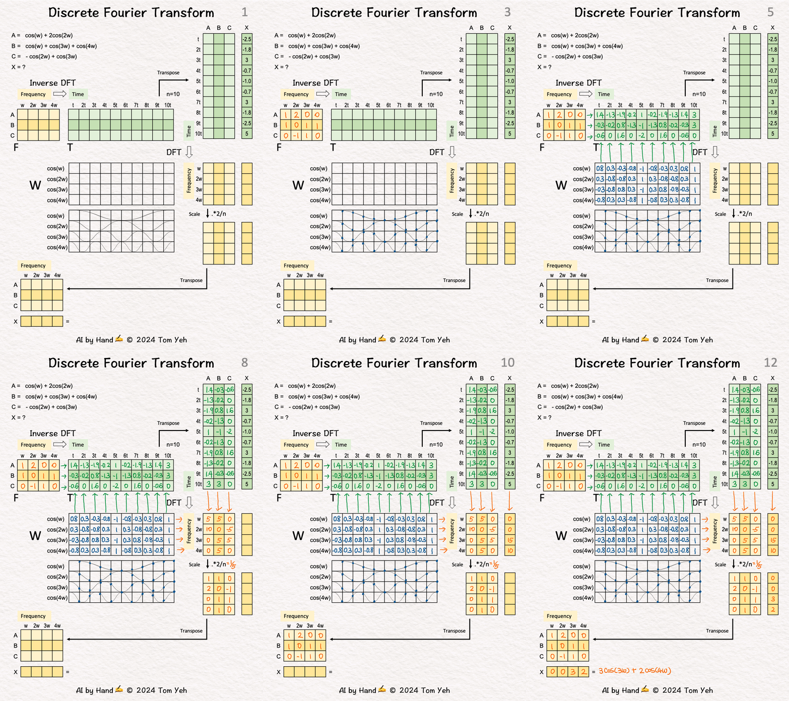
I developed this exercise to demonstrate that underneath such complexity, DFT is just a series of matrix multiplications you can calculate by hand. ✍️ Once you see that, it should not surprise you that a deep neural network, which is also a series of matrix multiplications, with activation functions in-between, can learn to perform DFT to process and analyze signals so effectively.
💡 Learned vs. Fixed: U-Net learns its filters from data to process a signal in the spatial domain. The DFT is the classical opposite, a fixed transform, designed by hand rather than learned, that views the same signal in the frequency domain as a combination of cosine waves.
How does DFT work?
Setup
Step 1 of 12: Given
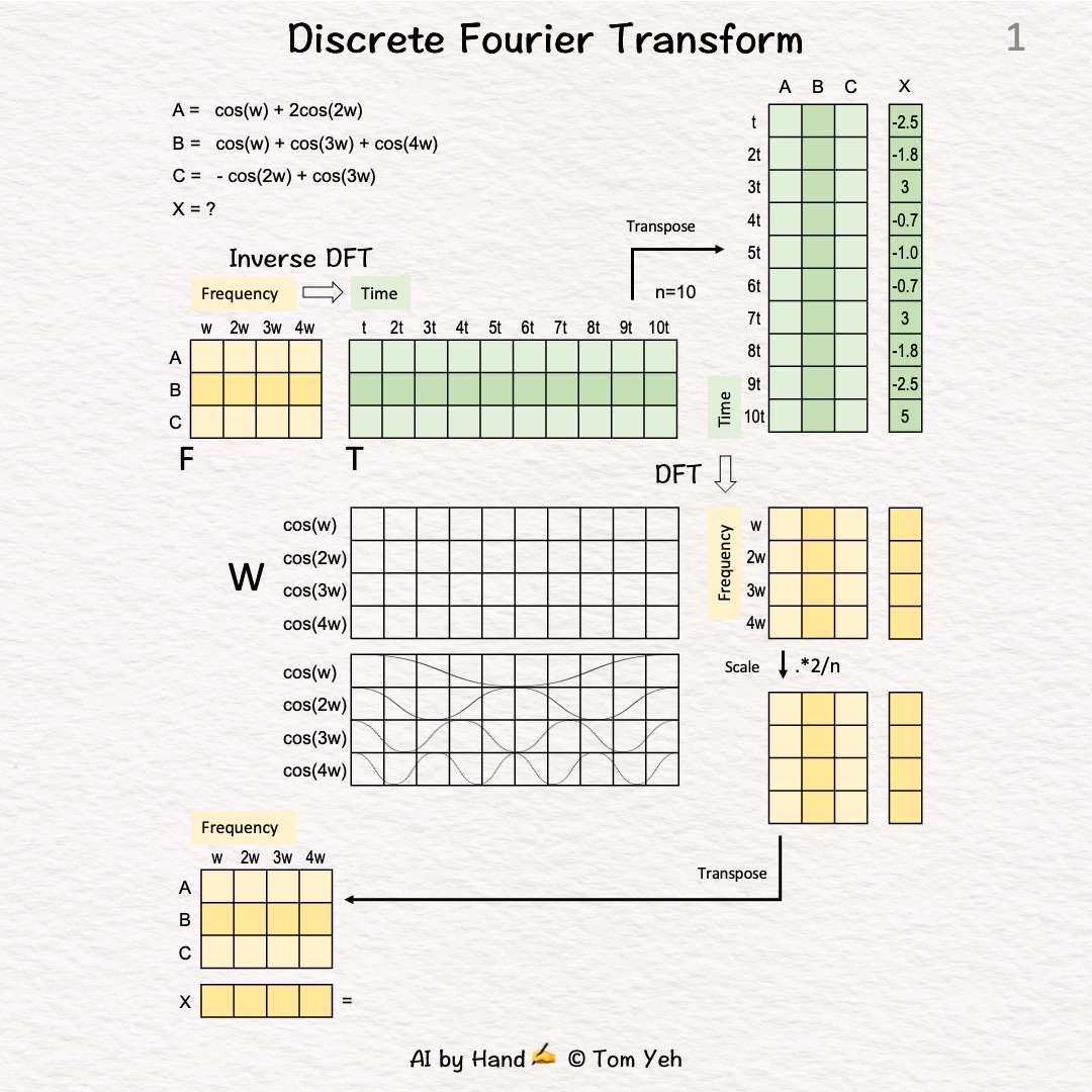
Signals A, B, and C in the 🟧 frequency domain:
A = cos(w) + 2cos(2w)
B = cos(w) + cos(3w) + cos(4w)
C = -cos(2w) + cos(3w)
Each signal is a weighed sum of four cosine waves at frequencies 1w, 2w, 3w, and 4w.
We will apply Inverse DFT to convert the signals to time domain representations, and then demonstrate DFT can convert back to their original frequency domain representations.
Signal X in the 🟩 time domain. X is sampled at 10 time points 1t, 2t, …, 10t:
X = [-2.5, -1.8, 3, -0.7, -1.0, -0.7, 3, -1.8, -2.5, 5]
Suppose X is also a weighted sum of the same four cosine waves, but we don’t already know their weights. We will apply DFT to discover them.
Step 2 of 12: Frequency Matrix (F)
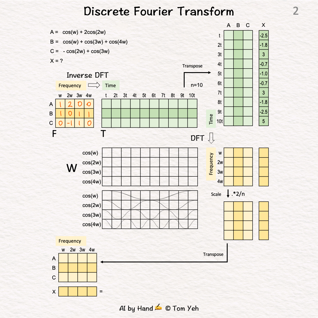
Write the coefficients of A, B, C as a matrix F. Each signal is a row. Each frequency is a column.
A → [1, 2, 0, 0]
B → [1, 0, 1, 1]
C → [0, -1, 1, 0]
Step 3 of 12: Cosine → Discrete
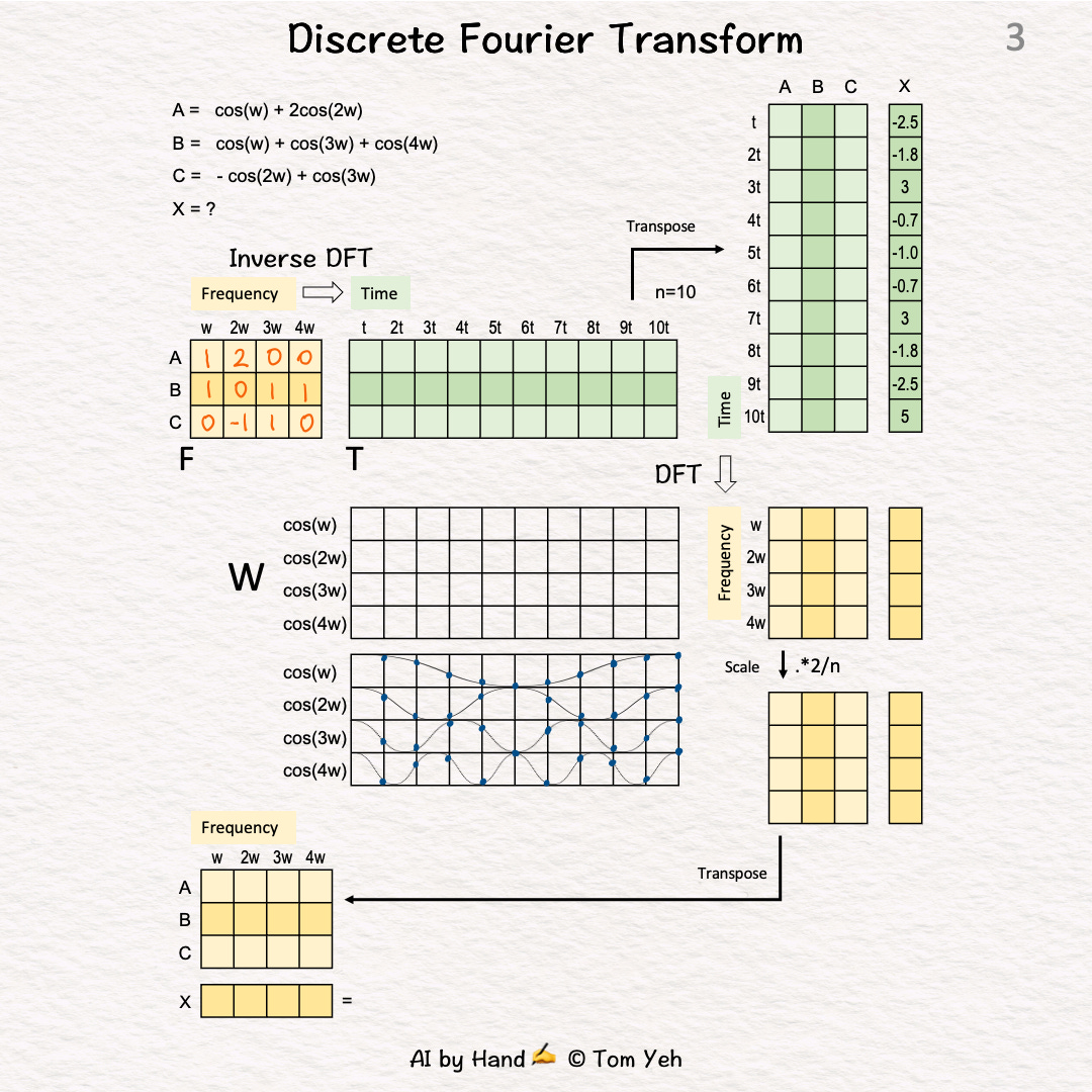
Sample from the continuous cosine waves at discrete time points 1t, 2t, 3t, to 10t.
Members read on: the rest of the walkthrough and the printable PDF.